
6个鲜为人知的Scikit-Learn功能,可以为您节省时间
对于许多学习数据科学的人来说,Scikit-Learn 往往是他们接触的第一个机器学习库。这是因为 Scikit-Learn 提供了各种对模型开发有用的 API,同时对初学者来说仍然易于使用。
尽管它们可能很有帮助,但 Scikit-Learn 的许多功能很少被探索,并具有未开发的潜力。本文将探讨六个可以为您节省时间的鲜为人知的功能。
1. 验证曲线
我们将要探讨的第一个函数是 Scikit-Learn 的 validation curve 函数。从名称中,您可以猜到它执行某种验证,但它执行的不仅仅是简单的验证。该函数会探索机器学习模型在特定超参数的各种值下的性能。
使用交叉验证方法,验证曲线函数会根据超参数值的范围评估训练和测试性能。该过程将产生两组分数,我们可以直观地进行比较。
让我们用样本数据尝试一下这个函数并可视化结果。首先,让我们加载样本数据并设置我们要探索的超参数范围。在这种情况下,我们将探索 SVC 模型在各种 gamma 超参数下的准确性表现。
|
1 2 3 4 5 6 7 8 9 10 11 12 13 14 15 16 17 18 |
import numpy as np import matplotlib.pyplot as plt from sklearn.model_selection import validation_curve from sklearn.svm import SVC from sklearn.datasets import load_iris data = load_iris() X, y = data.data, data.target param_range = np.logspace(-3, 3, 5) train_scores, test_scores = validation_curve( SVC(), X, y, param_name="gamma", param_range=param_range, cv=5, scoring="accuracy" ) |
执行上述代码后,您将获得两个分数:train_scores 和 test_scores。
它们都将分配类似下面的分数数组。
|
1 2 3 4 5 6 7 8 9 10 |
(array([[0.925 , 0.925 , 0.93333333, 0.925 , 0.9 ], [0.975 , 0.94166667, 0.975 , 0.96666667, 0.95833333], [0.975 , 0.98333333, 0.99166667, 0.99166667, 0.99166667], [1. , 1. , 1. , 1. , 1. ], [1. , 1. , 1. , 1. , 1. ]]), array([[0.86666667, 0.96666667, 0.83333333, 0.96666667, 0.93333333], [0.93333333, 0.96666667, 0.93333333, 0.93333333, 1. ], [0.96666667, 1. , 0.9 , 0.96666667, 1. ], [0.86666667, 0.73333333, 0.7 , 0.8 , 0.9 ], [0.46666667, 0.4 , 0.33333333, 0.4 , 0.4 ]])) |
我们可以使用类似下面的代码来可视化验证曲线。
|
1 2 3 4 5 6 7 8 9 |
plt.figure(figsize=(8, 6)) plt.plot(param_range, train_mean, label="训练分数", color="blue", marker="o") plt.plot(param_range, test_mean, label="交叉验证分数", color="green", marker="s") plt.xscale("log") plt.xlabel("Gamma") plt.ylabel("准确率") plt.title("SVC 验证曲线(gamma 参数)") plt.legend(loc="best") plt.show() |
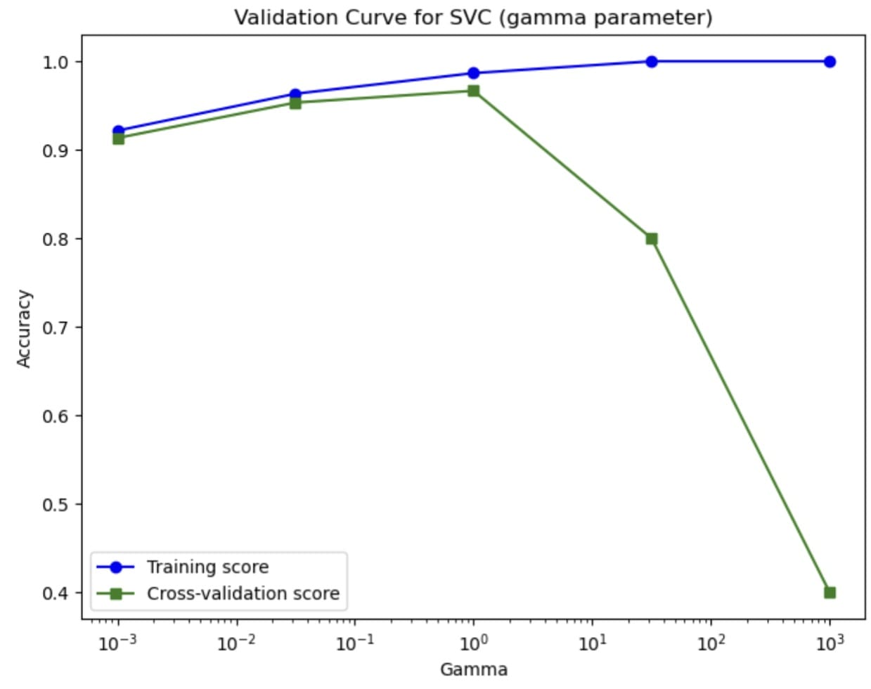
该曲线告诉我们超参数如何影响模型的性能。使用验证曲线,我们可以找到超参数的最佳值,并比依赖简单的训练-测试拆分更好地估计它。
尝试在您的模型开发过程中使用验证曲线来指导您开发最佳模型,并避免过拟合等问题。
2. 模型校准
当我们开发机器学习分类器模型时,我们需要记住,仅仅提供正确的分类预测是不够的;预测相关的概率也必须可靠。确保概率可靠的过程称为校准。
校准过程会调整模型的概率估计。该技术将概率推至反映预测的真实可能性,使其不过度自信或不自信。未校准的模型可能会预测事件的概率为 90%,而实际成功率却低得多,这意味着模型过于自信。这就是为什么我们需要校准模型。
通过校准模型,我们可以提高对模型预测的信任度,并告知用户模型的实际风险的实际估计。
让我们尝试使用 Scikit-Learn 进行校准过程。该库提供了一个诊断函数(calibration_curve)和一个模型校准类(CalibratedClassifierCV)。
我们将使用乳腺癌数据和逻辑回归模型作为基础。然后,我们将比较原始模型和校准模型的概率。
|
1 2 3 4 5 6 7 8 9 10 11 12 13 14 15 16 17 18 19 20 21 22 23 24 25 26 27 28 29 30 |
import numpy as np import matplotlib.pyplot as plt from sklearn.datasets import load_breast_cancer from sklearn.linear_model import LogisticRegression from sklearn.calibration import calibration_curve, CalibratedClassifierCV from sklearn.model_selection import train_test_split data = load_breast_cancer() X, y = data.data, data.target X_train, X_test, y_train, y_test = train_test_split(X, y, random_state=42) lr = LogisticRegression().fit(X_train, y_train) prob_pos_lr = lr.predict_proba(X_test)[:, 1] fraction_lr, mean_pred_lr = calibration_curve(y_test, prob_pos_lr, n_bins=10) calibrated_clf = CalibratedClassifierCV(lr, cv='prefit', method='isotonic') calibrated_clf.fit(X_train, y_train) prob_pos_calibrated = calibrated_clf.predict_proba(X_test)[:, 1] fraction_cal, mean_pred_cal = calibration_curve(y_test, prob_pos_calibrated, n_bins=10) plt.figure(figsize=(8, 6)) plt.plot(mean_pred_lr, fraction_lr, marker='o', label='原始 LR') plt.plot(mean_pred_cal, fraction_cal, marker='s', label='校准 LR(等渗)') plt.plot([0, 1], [0, 1], linestyle='--', label='完美校准') plt.xlabel("平均预测概率") plt.ylabel("阳性样本比例") plt.title("校准曲线比较") plt.legend(loc="upper left") plt.show() |

我们可以看到,校准后的逻辑回归比原始模型更接近完美校准模型。这意味着校准后的模型可以更好地估计实际风险,尽管它仍然不是理想的。
尝试使用校准方法来提高模型的预测能力。
3. 置换重要性
每当我们处理机器学习模型时,我们都会使用数据特征来提供预测结果。然而,并非所有特征都以相同的方式为预测做出贡献。
permutation_importance() 方法是通过随机置换(更改)特征值并评估置换后的模型性能来衡量特征对模型性能的贡献。如果模型性能下降,则该特征会影响模型;反之,如果模型性能不变,则表明该特征对于特定的模型性能可能不是那么有用。
该技术简单直观,使其有助于解释任何模型的内部决策过程。对于没有内置特征重要性方法的模型非常有益。
让我们用 Python 代码示例来尝试一下。我们将使用与我们之前的示例类似的数据和模型。
|
1 2 3 4 5 6 7 8 9 10 11 12 13 14 15 16 |
import numpy as np import matplotlib.pyplot as plt from sklearn.datasets import load_iris from sklearn.linear_model import LogisticRegression from sklearn.inspection import permutation_importance from sklearn.model_selection import train_test_split data = load_iris() X, y = data.data, data.target X_train, X_test, y_train, y_test = train_test_split(X, y, random_state=42) model = LogisticRegression() model.fit(X_train, y_train) result = permutation_importance(model, X_test, y_test, n_repeats=10, random_state=42, scoring='accuracy') |
通过上面的代码,我们得到了模型和置换重要性结果,我们将分析特征对模型的影响。让我们看一下置换重要性的平均值和标准差结果。
|
1 2 3 4 5 6 |
feature_names = data.feature_names importances = result.importances_mean std = result.importances_std for i, name in enumerate(feature_names): print(f"{name}: Mean importance = {importances[i]:.4f} (+/- {std[i]:.4f})") |
结果如下。
|
1 2 3 4 |
sepal length (cm): 平均重要性 = 0.0132 (+/- 0.0177) sepal width (cm): 平均重要性 = 0.0000 (+/- 0.0000) petal length (cm): 平均重要性 = 0.6000 (+/- 0.0805) petal width (cm): 平均重要性 = 0.1553 (+/- 0.0362) |
我们还可以可视化上面的结果,以便更好地理解模型性能。
|
1 2 3 4 |
plt.barh(feature_names, importances, xerr=std) plt.xlabel("准确率下降") plt.title("置换重要性") plt.show() |
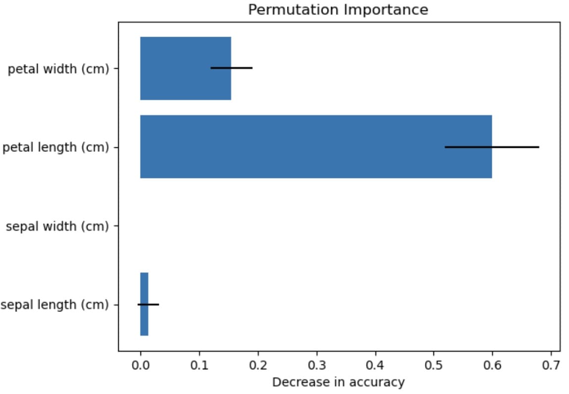
可视化显示,花瓣长度对特征性能影响最大,而花萼宽度没有影响。总有不确定性,这由标准差表示,但我们可以通过置换重要性技术得出花瓣长度影响最大的结论。
这是您可以在下一个项目中使用的简单特征重要性技术。
4. 特征哈希
在为数据科学建模处理特征时,我经常发现高维特征占用内存太多,影响了应用程序的整体性能。有许多方法可以提高性能,例如降维或特征选择。哈希方法是另一种可能很少使用但可能很有用的方法。
哈希是将数据转换为固定大小的稀疏数字矩阵。通过对每个特征应用哈希函数,可以将表示的特征映射到稀疏矩阵。我们将通过 FeatureHasher 使用哈希函数来计算对应于名称的矩阵列。
让我们用 Python 代码尝试一下。
|
1 2 3 4 5 6 7 8 9 10 11 12 13 14 15 |
import pandas as pd import seaborn as sns from sklearn.feature_extraction import FeatureHasher titanic = sns.load_dataset("titanic") titanic_sample = titanic[['sex', 'embarked', 'class']].dropna() data_dicts = titanic_sample.to_dict(orient='records') hasher = FeatureHasher(n_features=10, input_type='dict') hashed_features = hasher.transform(data_dicts) hashed_array = hashed_features.toarray() print("\nHashed feature matrix (dense format):\n", hashed_array) |
您将看到输出类似下面的内容。
|
1 2 3 4 5 6 7 8 |
哈希特征矩阵(密集格式): [[ 1. 0. 0. ... 0. -1. 0.] [-1. 0. 0. ... 0. 0. 0.] [ 1. 0. 0. ... 0. 0. 0.] ... [ 1. 0. 0. ... 0. 0. 0.] [-1. 0. 0. ... 0. -1. 0.] [ 1. 0. 0. ... 0. -1. 0.]] |
该数据集已表示为具有 10 个不同特征的稀疏矩阵。您可以指定所需的哈希特征数量,以平衡内存使用和信息丢失。
5. 鲁棒缩放器
真实世界的数据很少是干净的,而且往往充满了异常值。虽然异常值本身并没有错,并且可能提供有助于实际洞察的信息,但有时它会扭曲我们的模型结果。
有许多缩放异常值的技术,但有时它们会引入偏差。这就是为什么鲁棒缩放对于帮助预处理我们的数据很重要。鲁棒缩放器通过移除中位数并根据 IQR 进行缩放来转换数据,而不是使用均值和标准差。
鲁棒缩放器适用于只有少数极端位置异常值的情况。通过应用它,数据集是稳定的,并且不会受到异常值太多影响,这使得它对任何机器学习模型的开发都有用。
以下是使用鲁棒缩放器的示例。让我们使用 Iris 数据集示例,并在数据集中引入一个异常值。
|
1 2 3 4 5 6 7 8 9 10 11 12 13 |
import numpy as np import pandas as pd from sklearn.datasets import load_iris from sklearn.preprocessing import robust_scale import matplotlib.pyplot as plt iris = load_iris() X = iris.data outlier = np.array([[10, 10, 10, 10]]) X_out = np.vstack([X, outlier]) X_scaled = robust_scale(X_out) |
上面的代码可以轻松地缩放我们的异常值数据。如果您在处理异常值时遇到困难,请自行尝试。
6. 特征联合
特征联合是 Scikit-Learn 的一项功能,可在管道中组合多个特征转换。特征联合不是顺序转换相同的特征,而是同时将数据输入到几个转换器中,以提供所有转换后的特征。
这是一项有用的功能,其中需要不同的转换器来捕获数据的不同方面,并且它们需要存在于数据集中。一种转换器可能用于 PCA 技术,而其他转换器则使用鲁棒缩放。
让我们用下面的代码尝试一下。例如,我们可以创建 PCA 和多项式特征转换器。
|
1 2 3 4 5 6 7 8 9 10 11 12 13 14 15 16 17 18 19 |
import numpy as np from sklearn.datasets import load_iris 从 sklearn.分解 导入 PCA from sklearn.preprocessing import PolynomialFeatures from sklearn.pipeline import FeatureUnion data = load_iris() X, y = data.data, data.target pca = PCA(n_components=2) poly = PolynomialFeatures(degree=2, include_bias=False) union = FeatureUnion(transformer_list=[ ('pca', pca), ('poly', poly) ]) X_transformed = union.fit_transform(X) |
下面显示了转换后的特征的示例结果。
|
1 2 3 |
[-2.68412563 0.31939725 5.1 3.5 1.4 0.2 26.01 17.85 7.14 1.02 12.25 4.9 0.7 1.96 0.28 0.04 ] |
结果包含我们之前转换的 PCA 和多项式特征。
尝试试验各种转换,看看它们是否适合您的分析。
结论
Scikit-Learn 是许多数据科学家用来轻松开发数据模型的库。它易于使用,并提供了许多对我们的模型工作有用的功能,但其中许多功能似乎未被充分利用,尽管它们可以为您节省时间。
在本文中,我们探讨了其中六个未被充分利用的功能,从验证曲线到特征哈希,再到一个不易受异常值影响的鲁棒缩放器。希望您在此文中有所收获,并且希望这对您有所帮助!


我之前还不知道这些功能,感谢 Cornellius 提供的精彩内容。鲁棒缩放器确实激励我获取真实世界的数据,我渴望了解更多。祝好!😊
不客气!
最有趣的。我发现 probability_importance 与其他方法相比非常出色。