来自真实世界场景的数据集对于构建和测试机器学习模型至关重要。您可能只是想获得一些数据来实验算法。您也可能想通过建立一个基准来评估您的模型,或者使用不同的数据集来确定其弱点。有时,您还可能想创建合成数据集,通过向数据中添加噪声、相关性或冗余信息,在受控条件下测试您的算法。
在本帖中,我们将说明如何使用 Python 从不同来源获取一些真实世界的时间序列数据。我们还将使用 Python 的库创建合成时间序列数据。
完成本教程后,您将了解:
- 如何使用
pandas_datareader - 如何使用
requests库调用 Web 服务器的 API - 如何生成合成时间序列数据
通过我的新书 Python for Machine Learning 快速启动您的项目,其中包含分步教程以及所有示例的Python 源代码文件。
让我们开始吧。
Python 数据集处理指南
照片由 Mehreen Saeed 拍摄,部分权利保留
教程概述
本教程分为三个部分;它们是:
- 使用
pandas_datareader - 使用
requests库通过远程服务器的 API 获取数据 - 生成合成时间序列数据
使用 pandas-datareader 加载数据
本帖将依赖一些库。如果您的系统中尚未安装它们,可以使用 pip 进行安装
|
1 |
pip install pandas_datareader requests |
pandas_datareader 库允许您 从不同来源获取数据,包括用于金融市场数据的 Yahoo Finance、用于全球发展数据的 World Bank 以及用于经济数据的 St. Louis Fed。在本节中,我们将展示如何从不同来源加载数据。
在后台,pandas_datareader 实时从网上抓取您想要的数据,并将其组装成 pandas DataFrame。由于网页结构差异很大,每个数据源都需要不同的读取器。因此,pandas_datareader 只支持从有限数量的来源读取,主要是与金融和经济时间序列相关的来源。
获取数据非常简单。例如,我们知道苹果的股票代码是 AAPL,因此我们可以像下面这样从 Yahoo Finance 获取苹果股票的每日历史价格
|
1 2 3 4 5 6 |
import pandas_datareader as pdr # 从雅虎财经服务器读取苹果股票 shares_df = pdr.DataReader('AAPL', 'yahoo', start='2021-01-01', end='2021-12-31') # 查看读取的数据 print(shares_df) |
DataReader() 的调用需要第一个参数指定股票代码,第二个参数指定数据源。上面的代码会打印 DataFrame
|
1 2 3 4 5 6 7 8 9 10 11 12 13 14 15 |
最高价 最低价 开盘价 收盘价 成交量 调整后收盘价 日期 2021-01-04 133.610001 126.760002 133.520004 129.410004 143301900.0 128.453461 2021-01-05 131.740005 128.429993 128.889999 131.009995 97664900.0 130.041611 2021-01-06 131.050003 126.379997 127.720001 126.599998 155088000.0 125.664215 2021-01-07 131.630005 127.860001 128.360001 130.919998 109578200.0 129.952271 2021-01-08 132.630005 130.229996 132.429993 132.050003 105158200.0 131.073914 ... ... ... ... ... ... ... 2021-12-27 180.419998 177.070007 177.089996 180.330002 74919600.0 180.100540 2021-12-28 181.330002 178.529999 180.160004 179.289993 79144300.0 179.061859 2021-12-29 180.630005 178.139999 179.330002 179.380005 62348900.0 179.151749 2021-12-30 180.570007 178.089996 179.470001 178.199997 59773000.0 177.973251 2021-12-31 179.229996 177.259995 178.089996 177.570007 64062300.0 177.344055 [252 行 x 6 列] |
我们也可以用股票代码列表来获取多家公司的股票价格历史记录
|
1 2 3 |
companies = ['AAPL', 'MSFT', 'GE'] shares_multiple_df = pdr.DataReader(companies, 'yahoo', start='2021-01-01', end='2021-12-31') print(shares_multiple_df.head()) |
结果将是一个具有多级列的 DataFrame
|
1 2 3 4 5 6 7 8 9 10 11 12 13 14 15 16 17 18 19 |
属性 调整后收盘价 收盘价 \ 股票代码 AAPL MSFT GE AAPL MSFT 日期 2021-01-04 128.453461 215.434982 83.421600 129.410004 217.690002 2021-01-05 130.041611 215.642776 85.811905 131.009995 217.899994 2021-01-06 125.664223 210.051315 90.512833 126.599998 212.250000 2021-01-07 129.952286 216.028732 89.795753 130.919998 218.289993 2021-01-08 131.073944 217.344986 90.353485 132.050003 219.619995 ... 属性 成交量 股票代码 AAPL MSFT GE 日期 2021-01-04 143301900.0 37130100.0 9993688.0 2021-01-05 97664900.0 23823000.0 10462538.0 2021-01-06 155088000.0 35930700.0 16448075.0 2021-01-07 109578200.0 27694500.0 9411225.0 2021-01-08 105158200.0 22956200.0 9089963.0 |
由于 DataFrame 的结构,提取部分数据非常方便。例如,我们可以使用以下方法仅绘制某些日期的每日收盘价
|
1 2 3 4 5 6 7 8 9 10 11 12 13 14 15 16 |
import matplotlib.pyplot as plt import matplotlib.ticker as ticker # 绘制时间序列数据的通用例程 def plot_timeseries_df(df, attrib, ticker_loc=1, title='Timeseries', legend=''): fig = plt.figure(figsize=(15,7)) plt.plot(df[attrib], 'o-') _ = plt.xticks(rotation=90) plt.gca().xaxis.set_major_locator(ticker.MultipleLocator(ticker_loc)) plt.title(title) plt.gca().legend(legend) plt.show() plot_timeseries_df(shares_multiple_df.loc["2021-04-01":"2021-06-30"], "Close", ticker_loc=3, title="收盘价", legend=companies) |
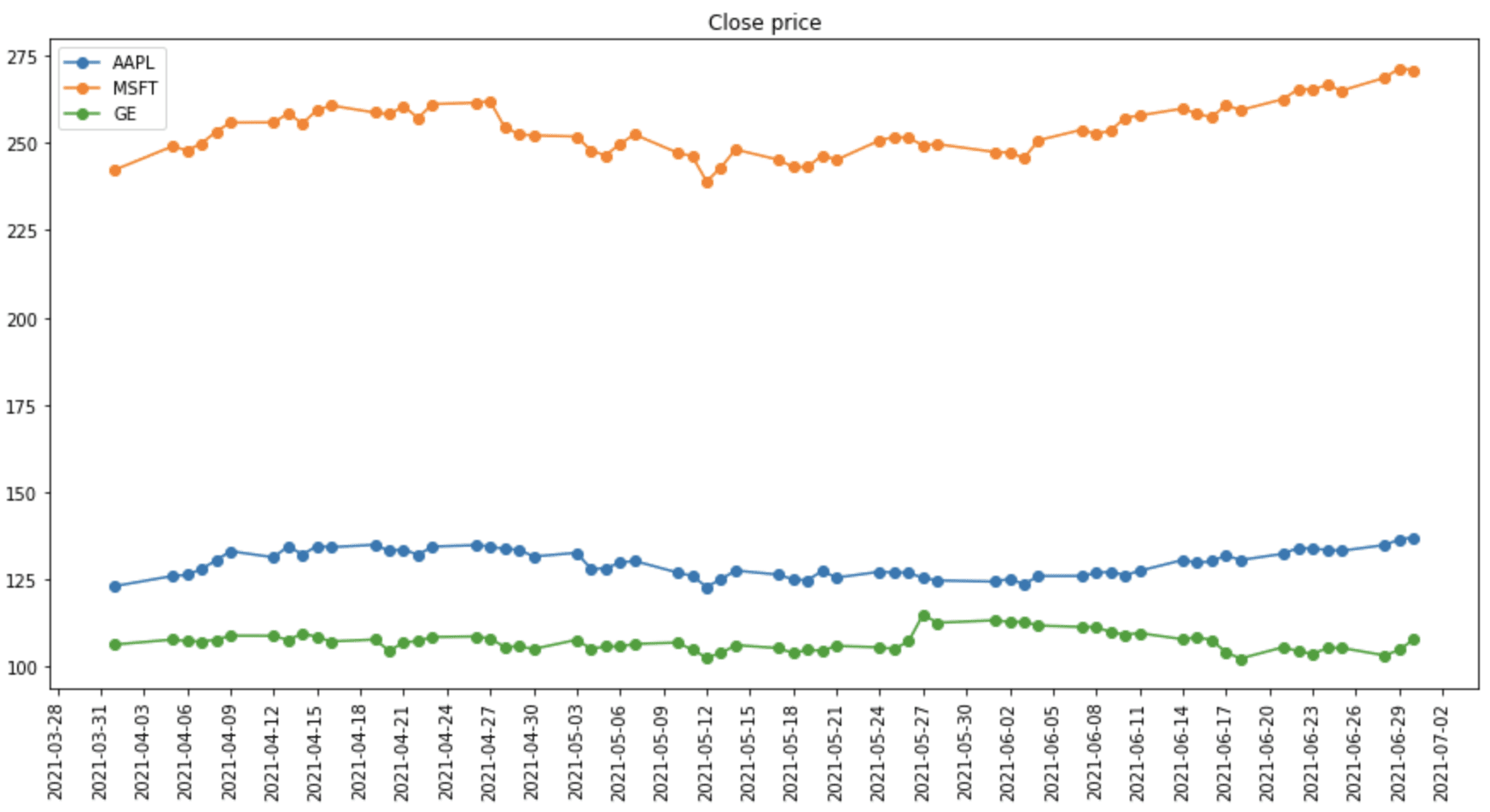
从 Yahoo Finance 获取的多只股票
完整代码如下:
|
1 2 3 4 5 6 7 8 9 10 11 12 13 14 15 16 17 18 19 20 |
import pandas_datareader as pdr import matplotlib.pyplot as plt import matplotlib.ticker as ticker companies = ['AAPL', 'MSFT', 'GE'] shares_multiple_df = pdr.DataReader(companies, 'yahoo', start='2021-01-01', end='2021-12-31') print(shares_multiple_df) def plot_timeseries_df(df, attrib, ticker_loc=1, title='Timeseries', legend=''): "通用例程,用于绘制时间序列数据" fig = plt.figure(figsize=(15,7)) plt.plot(df[attrib], 'o-') _ = plt.xticks(rotation=90) plt.gca().xaxis.set_major_locator(ticker.MultipleLocator(ticker_loc)) plt.title(title) plt.gca().legend(legend) plt.show() plot_timeseries_df(shares_multiple_df.loc["2021-04-01":"2021-06-30"], "Close", ticker_loc=3, title="收盘价", legend=companies) |
使用 pandas-datareader 从另一个数据源读取的语法是类似的。例如,我们可以从 美联储经济数据 (FRED) 读取经济时间序列。FRED 中的每个时间序列都由一个符号标识。例如,所有城市消费者的消费者价格指数是 CPIAUCSL,不包括食品和能源的所有项目的消费者价格指数是 CPILFESL,个人消费支出是 PCE。您可以从 FRED 的网页搜索和查找符号。
下面是如何获取两个消费者价格指数 CPIAUCSL 和 CPILFESL,并在图表中显示它们
|
1 2 3 4 5 6 7 8 9 10 11 12 13 14 |
import pandas_datareader as pdr import matplotlib.pyplot as plt # 从 FRED 读取数据并打印 fred_df = pdr.DataReader(['CPIAUCSL','CPILFESL'], 'fred', "2010-01-01", "2021-12-31") print(fred_df) # 在图中显示 2019-2021 年的数据 fig = plt.figure(figsize=(15,7)) plt.plot(fred_df.loc["2019":], 'o-') plt.xticks(rotation=90) plt.legend(fred_df.columns) plt.title("消费者价格指数") plt.show() |
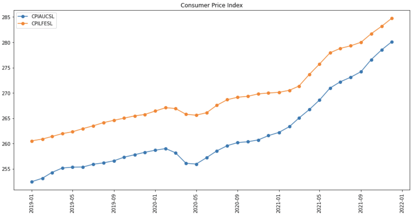
消费者价格指数图
从世界银行获取数据也很相似,但我们必须了解世界银行的数据更加复杂。通常,人口等数据系列既是时间序列,也具有国家维度。因此,我们需要指定更多参数来获取数据。
使用 pandas_datareader,我们有一个针对世界银行的特定 API 集。指标的符号可以从 世界银行开放数据中查找,或使用以下方式搜索
|
1 2 3 4 |
from pandas_datareader import wb matches = wb.search('total.*population') print(matches[["id","name"]]) |
search() 函数接受一个正则表达式字符串(例如,上面的 .* 表示任意长度的字符串)。这将打印
|
1 2 3 4 5 6 7 8 9 10 11 12 13 14 |
id name 24 1.1_ACCESS.ELECTRICITY.TOT 电力接入 (占 总 人口 % ) 164 2.1_ACCESS.CFT.TOT 清洁燃料和烹饪技术接入... 1999 CC.AVPB.PTPI.AI 低于 1.90 美元的人口比例(占总人口 % )... 2000 CC.AVPB.PTPI.AR 低于 1.90 美元的人口比例 (占总人口 % )... 2001 CC.AVPB.PTPI.DI 低于 1.90 美元的人口比例 (占总人口 % )... ... ... ... 13908 SP.POP.TOTL.FE.ZS 人口, 女性 (占 总人口 % ) 13912 SP.POP.TOTL.MA.ZS 人口, 男性 (占 总人口 % ) 13938 SP.RUR.TOTL.ZS 农村人口 (占 总人口 % ) 13958 SP.URB.TOTL.IN.ZS 城市人口 (占 总人口 % ) 13960 SP.URB.TOTL.ZS 城市地区人口百分比 (占 % )... [137 行 x 2 列] |
其中 id 列是时间序列的符号。
我们可以通过指定 ISO-3166-1 国家代码来读取特定国家的数据。但世界银行也包含非国家聚合(例如,南亚),因此虽然 pandas_datareader 允许我们使用字符串 “all” 来表示所有国家,但我们通常不使用它。下面是如何获取世界银行所有国家和地区的列表
|
1 2 3 4 |
import pandas_datareader.wb as wb countries = wb.get_countries() print(countries) |
|
1 2 3 4 5 6 7 8 9 10 11 12 |
iso3c iso2c name region adminregion incomeLevel lendingType capitalCity longitude latitude 0 ABW AW 阿鲁巴 拉丁美洲和加勒比 高收入 未分类 奥拉涅斯塔德 -70.0167 12.5167 1 AFE ZH 非洲东部 聚合体 聚合体 聚合体 NaN NaN 2 AFG AF 阿富汗 南亚 南亚 低收入 IDA 喀布尔 69.1761 34.5228 3 AFR A9 非洲 聚合体 聚合体 聚合体 NaN NaN 4 AFW ZI 非洲西部 聚合体 聚合体 聚合体 NaN NaN .. ... ... ... ... ... ... ... ... ... ... 294 XZN A5 撒哈拉以南非洲 聚合体 聚合体 聚合体 NaN NaN 295 YEM YE 也门,也门共和国 中东和北非 中东和北非 低收入 IDA 萨那 44.2075 15.3520 296 ZAF ZA 南非 撒哈拉以南非洲 撒哈拉以南非洲 中上收入 IBRD 比勒陀利亚 28.1871 -25.7460 297 ZMB ZM 赞比亚 撒哈拉以南非洲 撒哈拉以南非洲 下中等收入 IDA 卢萨卡 28.2937 -15.3982 298 ZWE ZW 津巴布韦 撒哈拉以南非洲 撒哈拉以南非洲 下中等收入 混合 哈拉雷 31.0672 -17.8312 |
下面是如何获取 2020 年所有国家的人口,并用条形图显示排名前 25 的国家。当然,我们也可以通过指定不同的 start 和 end 年份来获取跨年份的人口数据
|
1 2 3 4 5 6 7 8 9 10 11 12 13 14 15 16 17 18 19 20 21 22 23 24 |
import pandas_datareader.wb as wb import pandas as pd import matplotlib.pyplot as plt # 获取不包含聚合体的两位国家代码列表 countries = wb.get_countries() countries = list(countries[countries.region != "Aggregates"]["iso2c"]) # 读取 2020 年各国的总人口数据 (SP.POP.TOTL) population_df = wb.download(indicator="SP.POP.TOTL", country=countries, start=2020, end=2020) # 按人口排序,然后取前 25 个国家,并将索引(即国家)作为一列 population_df = (population_df.dropna() .sort_values("SP.POP.TOTL") .iloc[-25:] .reset_index()) # 绘制人口数,单位为百万 fig = plt.figure(figsize=(15,7)) plt.bar(population_df["country"], population_df["SP.POP.TOTL"]/1e6) plt.xticks(rotation=90) plt.ylabel("百万人口") plt.title("人口") plt.show() |
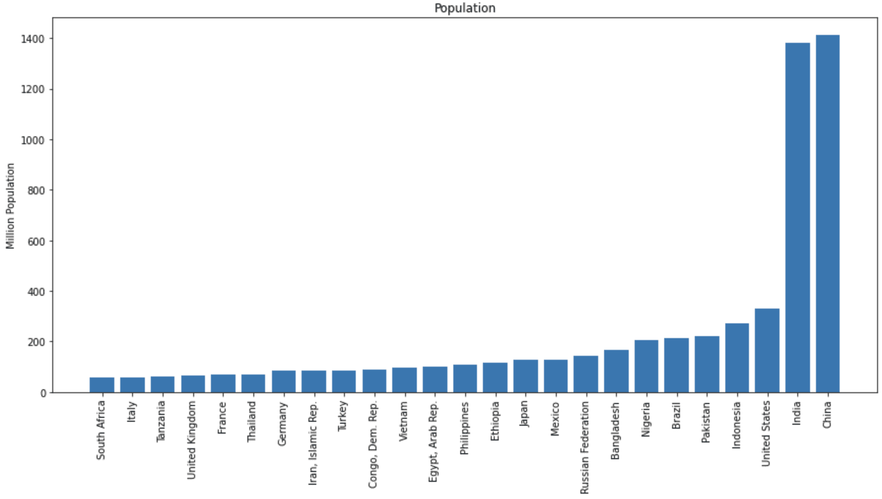
不同国家总人口的条形图
想开始学习机器学习 Python 吗?
立即参加我为期7天的免费电子邮件速成课程(附示例代码)。
点击注册,同时获得该课程的免费PDF电子书版本。
使用 Web API 获取数据
除了使用 the pandas_datareader 库之外,有时您也可以选择直接调用其 Web API,无需任何身份验证,直接从 Web 数据服务器获取数据。这可以使用 Python 的标准库 urllib.requests 来完成,或者您也可以使用 requests 库获得更简单的接口。
世界银行就是一个 Web API 可以免费访问的例子,因此我们可以轻松地读取不同格式的数据,例如 JSON、XML 或纯文本。 世界银行数据存储库 API 页面描述了各种 API 及其相应参数。为了重现之前不使用 pandas_datareader 的示例,我们首先构造一个 URL 来读取所有国家/地区的列表,以便找到不是聚合体的国家代码。然后,我们可以使用以下参数构造一个查询 URL
country参数,值为allindicator参数,值为SP.POP.TOTLdate参数,值为2020format参数,值为json
当然,您可以尝试不同的 指标。默认情况下,世界银行每页返回 50 个条目,我们需要逐页查询才能获取所有数据。我们可以增大每页大小,一次性获取所有数据。下面是如何以 JSON 格式获取国家列表并收集国家代码
|
1 2 3 4 5 6 7 8 9 10 11 12 13 14 15 |
import requests # 创建国家列表的查询 URL,默认每页只返回 50 个条目 url = "http://api.worldbank.org/v2/country/all?format=json&per_page=500" response = requests.get(url) # 预期正确的查询结果返回HTTP状态码200 print(response.status_code) # 获取JSON格式的响应 header, data = response.json() print(header) # 收集排除汇总信息的3字母国家代码列表 countries = [item["id"] for item in data if item["region"]["value"] != "Aggregates"] print(countries) |
它将打印HTTP状态码、头部信息以及国家代码列表,如下所示
|
1 2 3 |
200 {'page': 1, 'pages': 1, 'per_page': '500', 'total': 299} ['ABW', 'AFG', 'AGO', 'ALB', ..., 'YEM', 'ZAF', 'ZMB', 'ZWE'] |
从头部信息,我们可以确认我们已经获取了所有数据(第1页,共1页)。然后,我们可以像下面这样获取所有的人口数据
|
1 2 3 4 5 6 7 8 9 10 11 12 13 14 15 |
... # 创建2020年所有国家总人口的查询URL arguments = { "country": "all", "indicator": "SP.POP.TOTL", "date": "2020:2020", "format": "json" } url = "http://api.worldbank.org/v2/country/{country}/" \ "indicator/{indicator}?date={date}&format={format}&per_page=500" query_population = url.format(**arguments) response = requests.get(query_population) # 获取JSON格式的响应 header, population_data = response.json() |
您应该查阅世界银行API文档以了解如何构建URL的详细信息。例如,日期语法2020:2021表示开始和结束年份,额外的参数page=3将为您提供多页结果中的第三页。获取数据后,我们可以仅筛选出非汇总国家的数据,将其放入pandas DataFrame进行排序,然后绘制条形图
|
1 2 3 4 5 6 7 8 9 10 11 12 13 14 15 16 17 18 |
... # 筛选国家,排除汇总信息 population = [] for item in population_data: if item["countryiso3code"] in countries: name = item["country"]["value"] population.append({"country":name, "population": item["value"]}) # 创建DataFrame用于排序和过滤 population = pd.DataFrame.from_dict(population) population = population.dropna().sort_values("population").iloc[-25:] # 绘制条形图 fig = plt.figure(figsize=(15,7)) plt.bar(population["country"], population["population"]/1e6) plt.xticks(rotation=90) plt.ylabel("百万人口") plt.title("人口") plt.show() |
图形应该与之前完全相同。但您可以看到,使用pandas_datareader可以使代码更简洁,隐藏了底层操作。
把所有东西放在一起,下面是完整的代码。
|
1 2 3 4 5 6 7 8 9 10 11 12 13 14 15 16 17 18 19 20 21 22 23 24 25 26 27 28 29 30 31 32 33 34 35 36 37 38 39 40 41 42 43 44 45 46 47 48 49 50 51 52 53 |
import pandas as pd import matplotlib.pyplot as plt import requests # 创建国家列表的查询 URL,默认每页只返回 50 个条目 url = "http://api.worldbank.org/v2/country/all?format=json&per_page=500" response = requests.get(url) # 预期正确的查询结果返回HTTP状态码200 print(response.status_code) # 获取JSON格式的响应 header, data = response.json() print(header) # 收集排除汇总信息的3字母国家代码列表 countries = [item["id"] for item in data if item["region"]["value"] != "Aggregates"] print(countries) # 创建2020年所有国家总人口的查询URL arguments = { "country": "all", "indicator": "SP.POP.TOTL", "date": 2020, "format": "json" } url = "http://api.worldbank.org/v2/country/{country}/" \ "indicator/{indicator}?date={date}&format={format}&per_page=500" query_population = url.format(**arguments) response = requests.get(query_population) print(response.status_code) # 获取JSON格式的响应 header, population_data = response.json() print(header) # 筛选国家,排除汇总信息 population = [] for item in population_data: if item["countryiso3code"] in countries: name = item["country"]["value"] population.append({"country":name, "population": item["value"]}) # 创建DataFrame用于排序和过滤 population = pd.DataFrame.from_dict(population) population = population.dropna().sort_values("population").iloc[-25:] # 绘制条形图 fig = plt.figure(figsize=(15,7)) plt.bar(population["country"], population["population"]/1e6) plt.xticks(rotation=90) plt.ylabel("百万人口") plt.title("人口") plt.show() |
使用NumPy创建合成数据
有时,我们可能不想在项目中使用真实世界的数据,因为我们需要一些现实中可能不会发生但特定的东西。一个典型的例子是使用理想的时间序列数据来测试模型。在本节中,我们将学习如何创建合成自回归(AR)时间序列数据。
numpy.random库可用于从不同分布创建随机样本。randn()方法生成具有零均值和单位方差的标准正态分布数据。
在n阶AR(n)模型中,时间步t的值$x_t$取决于前n个时间步的值。即:
$$
x_t = b_1 x_{t-1} + b_2 x_{t-2} + … + b_n x_{t-n} + e_t
$$
其中$b_i$是$x_t$不同**滞后**的系数,误差项$e_t$预计遵循正态分布。
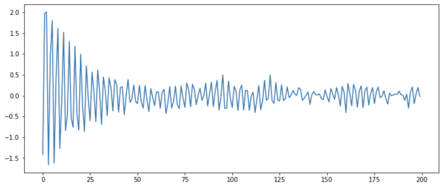
理解了这个公式,我们可以在下面的示例中生成一个AR(3)时间序列。我们首先使用randn()生成序列的前3个值,然后迭代应用上述公式生成下一个数据点。然后,使用randn()函数再次添加一个误差项,该误差项受预定义的noise_level约束
|
1 2 3 4 5 6 7 8 9 10 11 12 13 14 15 16 17 18 19 20 |
import numpy as np # 预定义参数 ar_n = 3 # AR(n)数据的阶数 ar_coeff = [0.7, -0.3, -0.1] # 系数 b_3, b_2, b_1 noise_level = 0.1 # 添加到AR(n)数据的噪声水平 length = 200 # 要生成的数据点数量 # 随机初始值 ar_data = list(np.random.randn(ar_n)) # 生成其余值 for i in range(length - ar_n): next_val = (np.array(ar_coeff) @ np.array(ar_data[-3:])) + np.random.randn() * noise_level ar_data.append(next_val) # 绘制时间序列 fig = plt.figure(figsize=(12,5)) plt.plot(ar_data) plt.show() |
上面的代码将生成如下图形
但是,我们可以通过首先将数据转换为pandas DataFrame,然后添加时间作为索引来进一步添加时间轴
|
1 2 3 4 5 6 7 8 9 10 11 12 |
... # 将数据转换为pandas DataFrame synthetic = pd.DataFrame({"AR(3)": ar_data}) synthetic.index = pd.date_range(start="2021-07-01", periods=len(ar_data), freq="D") # 绘制时间序列 fig = plt.figure(figsize=(12,5)) plt.plot(synthetic.index, synthetic) plt.xticks(rotation=90) plt.title("AR(3)时间序列") plt.show() |
之后,我们将得到以下图形
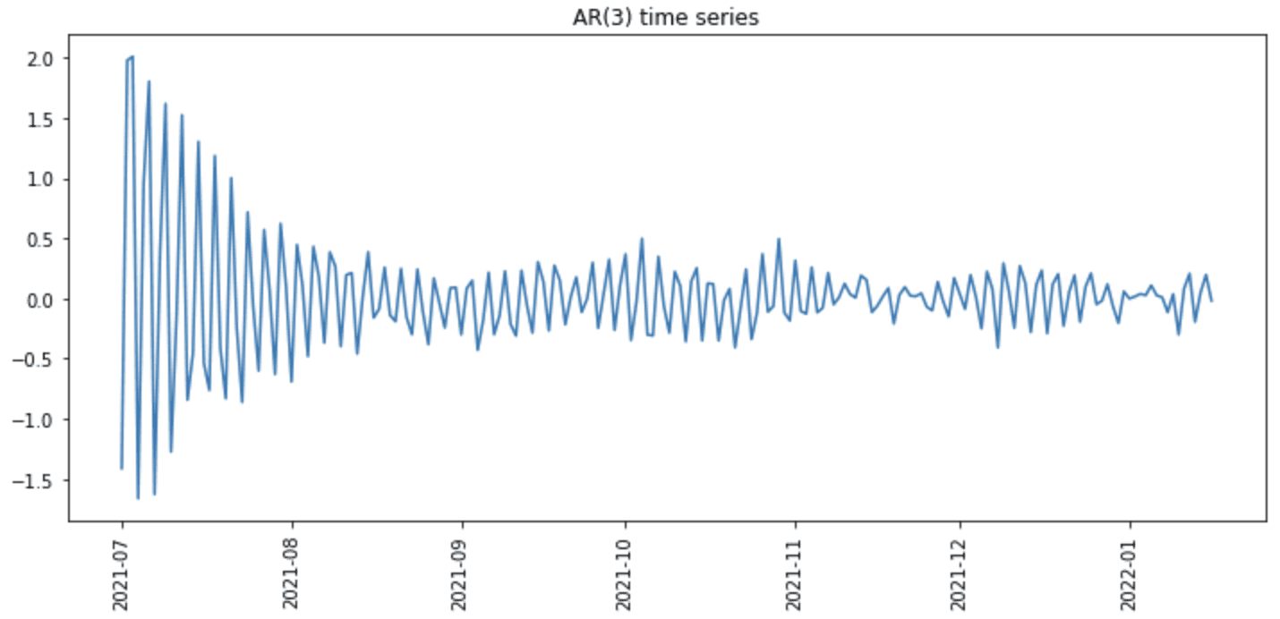
合成时间序列图
使用类似的技术,我们还可以生成纯随机噪声(即AR(0)序列)、ARIMA时间序列(即具有误差项系数的时间序列)或布朗运动时间序列(即随机噪声的累加和)。
进一步阅读
如果您想深入了解,本节提供了更多关于该主题的资源。
库
数据源
书籍
- 《像计算机科学家一样思考 Python》 作者:Allen B. Downey
- Mark Summerfield著《Python 3编程:Python语言完全入门》
- Wes McKinney著《Python for Data Analysis》(第二版)
总结
在本教程中,您探索了在Python中获取数据或生成合成时间序列数据的各种选项。
具体来说,你学到了:
- 如何使用
pandas_datareader从不同数据源获取金融数据 - 如何使用
requests库调用API从不同的Web服务器获取数据 - 如何使用NumPy的随机数生成器生成合成时间序列数据
您对本帖讨论的主题有任何疑问吗?请在下方评论区提问,我会尽力回答。
掌握机器学习 Python!

更自信地用 Python 编写代码
...从学习实用的 Python 技巧开始
在我的新电子书中探索如何实现
用于机器学习的 Python
它提供自学教程和数百个可运行的代码,为您提供包括以下技能:
调试、性能分析、鸭子类型、装饰器、部署等等...

")


Mehreen,
晚上好!这太棒了,尤其是关于开发合成时间序列数据的最后一部分。我处理的是时间序列数据序列,并且一直在使用一种劣等的方法来开发合成数据。虽然时间序列数据本身就很复杂,但时间序列序列会带来额外的复杂性,我可以将其作为指导,使我的数据更加健壮。非常感谢您发布这个!
保重,
Jeremy
关于将时间作为索引添加的先前错误的版本信息
Python: 3.9.7 (default, Sep 16 2021, 13:09:58)
[GCC 7.5.0]
scipy: 1.7.3
numpy: 1.21.2
matplotlib: 3.5.1
pandas: 1.4.1
statsmodels: 0.13.2
sklearn: 1.0.2
theano: 1.0.5
tensorflow: 2.4.1
keras: 2.4.3
你好……请说明您遇到错误的哪个代码列表。
嗨,我收到一个remotedata错误消息!
我可以在哪里共享日志?
嗨 Amit……你能发布确切的错误消息吗?
你好,
在尝试获取数据时,我收到以下错误消息。
你能支持一下吗?
错误消息:ConnectionError: HTTPSConnectionPool(host=’finance.yahoo.com’, port=443): Max retries exceeded with url: /quote/AAPL/history?period1=1609462800&period2=1640998799&interval=1d&frequency=1d&filter=history (Caused by NewConnectionError(‘: Failed to establish a new connection: [Errno 11001] getaddrinfo failed’))
嗨 F.S……以下讨论可能会引起您的兴趣
https://stackoverflow.com/questions/63881566/python-connectionerror-httpsconnectionpoolhost-finance-yahoo-com-port-443