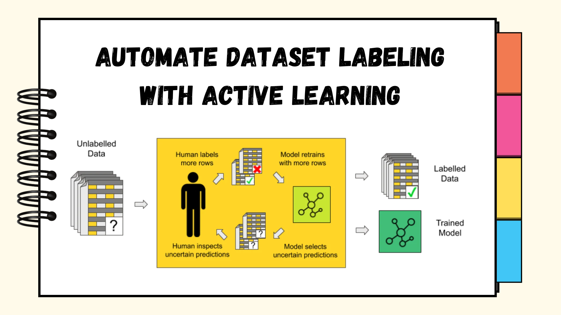
图片来源:作者 | Canva & Knime插图
几年前,训练人工智能模型需要海量的标注数据。手动收集和标注这些数据既耗时又昂贵。但幸运的是,我们从那时起已经取得了长足的进步,现在我们拥有了更强大的工具和技术来帮助我们自动化这个标注过程。其中最有效的方法之一是什么?**主动学习。**
在本文中,我们将介绍主动学习的概念、工作原理,并分享一个循序渐进的实现过程,介绍如何使用这种方法来自动化文本分类任务的数据集标注。
什么是主动学习及其工作原理?
在典型的监督学习设置中会发生什么?你有一个完全标注的数据集,你训练了一个模型,其中每个数据点都有一个已知的输出。对吗?但遗憾的是,在许多现实场景中,获取所有这些标签可能非常困难。这时主动学习就派上用场了。
它是一种半监督学习的形式,算法可以实际寻求帮助——通过查询人类标注者或“预言家”来标注特定的数据点。但这里的关键是:主动学习不是随机选择数据点,而是选择对改进模型最有用的数据点。这些通常是模型最不确定的样本。一旦这些不确定的数据点被标注(通常由人类完成),它们就会被反馈给模型以重新训练它。这个循环会不断重复——每次都以最少的人工输入来改进模型。
这是来自 KNIME Blog 的一张图,总结了它的工作原理
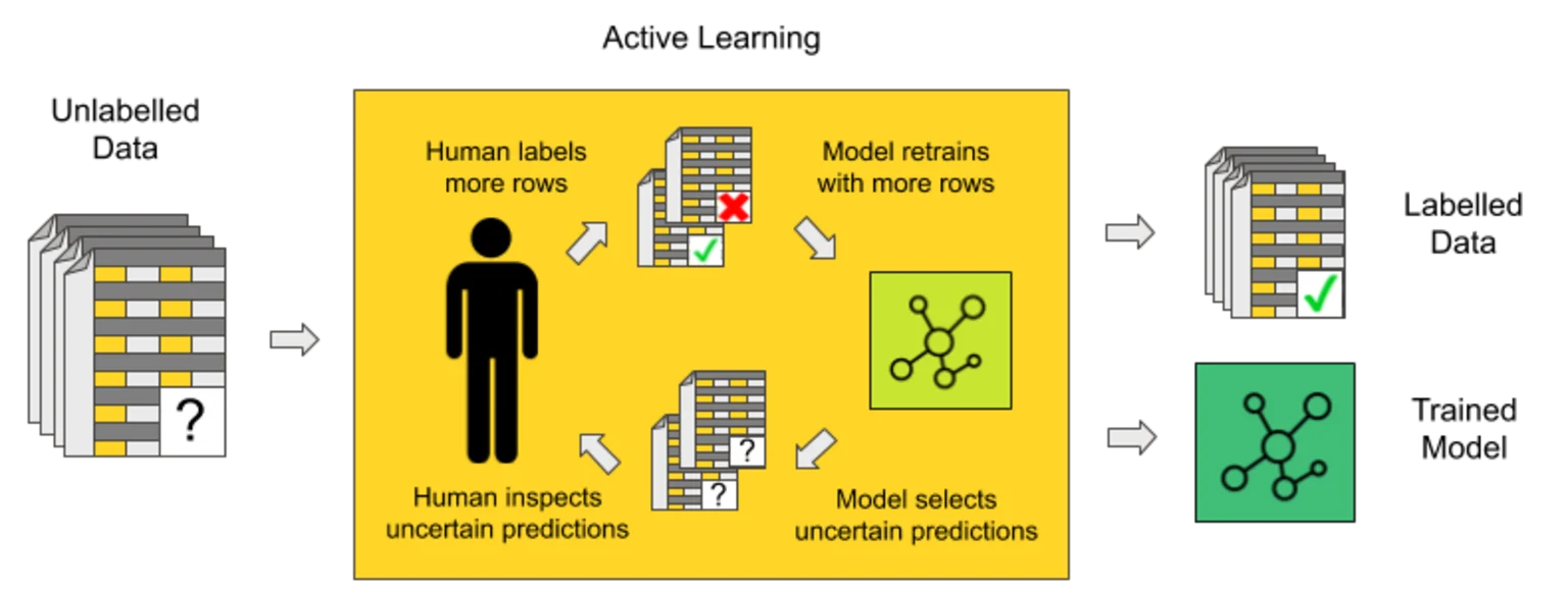
KNIME Blog – 主动学习工作原理
主动学习中的关键概念
让我们快速回顾一些关键概念和术语——这样在稍后的实现阶段使用它们时就不会感到困惑。
- 未标注池: 模型尚未见过的数据点池
- 已标注数据: 模型已从中学习的数据集,其中包含人类提供的标签
- 标注预言家: 为选定的数据点提供标签的外部来源或人类专家。
- 查询策略: 模型选择要标注的数据点的方法。常见策略包括
- 不确定性采样: 选择模型最不确定的实例(即模型预测的熵值较高)
- 随机采样: 随机选择数据点进行标注
- 多样性采样: 选择与现有已标注数据不同的样本,以提高特征空间的覆盖率
- 委员会查询: 使用多个模型对分歧最大的样本进行投票
- 预期模型变化: 识别在标注后对当前模型参数影响最大的样本
- 预期误差减少: 选择能最小化未标注池上预期误差的样本
文本分类任务的主动学习实践实现
为了更好地理解主动学习的实际应用,让我们通过一个例子来学习如何使用它来改进文本分类模型,该模型使用新闻文章数据集。该数据集包含两个类别的新闻:无神论和基督教,用于二元分类。我们的目标是训练一个分类器来预测这两个类别,但最初我们只标注一小部分数据,其余数据将根据不确定性或随机性进行查询标注。你可以根据数据集的性质和你的目标选择任何一种。
步骤 1:设置和初始数据准备
我们将首先安装必要的库并加载数据集。为此,我们将使用 20 newsgroups 数据集的一个子集,并将数据分成训练池和测试集。
|
1 2 3 4 5 6 7 8 9 10 11 12 13 14 15 16 17 18 19 20 21 22 23 24 25 26 27 28 29 30 31 32 33 |
# 安装所需的包 pip install scikit-learn numpy pandas matplotlib import numpy as np import pandas as pd from sklearn.feature_extraction.text import TfidfVectorizer from sklearn.linear_model import LogisticRegression from sklearn.metrics import accuracy_score import matplotlib.pyplot as plt import random from sklearn.datasets import fetch_20newsgroups # 为了可复现性 random.seed(42) np.random.seed(42) # 加载 20 newsgroups 数据集的一个子集(二元分类) categories = ['alt.atheism', 'soc.religion.christian'] newsgroups = fetch_20newsgroups(subset='train', categories=categories, remove=('headers', 'footers', 'quotes')) # 创建特征和标签 X = newsgroups.data y = newsgroups.target # 分割为训练集和测试集 from sklearn.model_selection import train_test_split X_pool, X_test, y_pool, y_test = train_test_split(X, y, test_size=0.2, random_state=42) # 初始化向量器 vectorizer = TfidfVectorizer(max_features=5000) # 将测试数据转换为 TF-IDF 特征 X_test_tfidf = vectorizer.fit_transform(X_test) |
步骤 2:实现主动学习函数
现在,我们定义主动学习循环中的关键函数。这些函数包括不确定性采样、随机采样和用于跟踪模型性能的评估函数。
|
1 2 3 4 5 6 7 8 9 10 11 12 13 14 15 16 17 18 19 20 21 |
def uncertainty_sampling(model, X_unlabeled, n_samples=10): """选择不确定性最高的样本。""" # 获取概率预测 probas = model.predict_proba(X_unlabeled) # 计算不确定性(接近 0.5 的概率) uncertainty = np.abs(probas[:, 0] - 0.5) # 获取最不确定样本的索引 uncertain_indices = np.argsort(uncertainty)[:n_samples] return uncertain_indices def random_sampling(X_unlabeled, n_samples=10): """随机选择样本。""" return np.random.choice(len(X_unlabeled), n_samples, replace=False) def evaluate_model(model, X_test, y_test): """在测试数据上评估模型。""" y_pred = model.predict(X_test) return accuracy_score(y_test, y_pred) |
步骤 3:实现主动学习循环
现在,我们为指定的迭代次数实现主动学习循环,模型在此过程中选择样本、获取标注,然后重新训练模型。我们将比较不确定性采样和随机采样,看看哪种策略在测试集上的表现更好。
|
1 2 3 4 5 6 7 8 9 10 11 12 13 14 15 16 17 18 19 20 21 22 23 24 25 26 27 28 29 30 31 32 33 34 35 36 37 38 39 40 41 42 43 44 45 46 47 48 49 50 51 52 53 54 55 56 57 58 59 60 61 62 63 64 65 66 |
def run_experiment(sampling_strategy, X_pool, y_pool, X_test, y_test, initial_samples=20, batch_size=10, iterations=10): """使用指定的采样策略运行主动学习实验。""" # 复制池数据以避免修改原始数据 X_pool_copy = X_pool.copy() y_pool_copy = y_pool.copy() # 向量化初始池数据 X_pool_tfidf = vectorizer.transform(X_pool_copy) # 随机选择初始样本 initial_indices = np.random.choice(len(X_pool_copy), initial_samples, replace=False) # 创建初始标注数据集 X_labeled = X_pool_tfidf[initial_indices] y_labeled = np.array(y_pool_copy)[initial_indices] # 创建未标注数据掩码 labeled_mask = np.zeros(len(X_pool_copy), dtype=bool) labeled_mask[initial_indices] = True # 初始化模型 model = LogisticRegression(random_state=42) # 初始化结果跟踪 accuracies = [] num_labeled = [] # 训练初始模型 model.fit(X_labeled, y_labeled) accuracies.append(evaluate_model(model, X_test_tfidf, y_test)) num_labeled.append(initial_samples) # 主动学习循环 for i in range(iterations): # 获取未标注数据 X_unlabeled = X_pool_tfidf[~labeled_mask] # 选择要标注的样本 if sampling_strategy == 'uncertainty': # 对于不确定性采样,我们需要当前模型 indices_to_label_relative = uncertainty_sampling(model, X_unlabeled, batch_size) # 转换为绝对索引 unlabeled_indices = np.where(~labeled_mask)[0] indices_to_label = unlabeled_indices[indices_to_label_relative] else: # 随机采样 unlabeled_indices = np.where(~labeled_mask)[0] indices_to_label = np.random.choice(unlabeled_indices, batch_size, replace=False) # 更新标注掩码 labeled_mask[indices_to_label] = True # 更新已标注数据集 X_labeled = X_pool_tfidf[labeled_mask] y_labeled = np.array(y_pool_copy)[labeled_mask] # 重新训练模型 model.fit(X_labeled, y_labeled) # 评估并跟踪结果 accuracy = evaluate_model(model, X_test_tfidf, y_test) accuracies.append(accuracy) num_labeled.append(np.sum(labeled_mask)) return num_labeled, accuracies |
步骤 4:运行实验并可视化结果
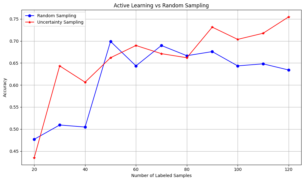
最后,我们将使用不确定性采样和随机采样策略运行我们的实验,并可视化准确性结果随时间的变化。
|
1 2 3 4 5 6 7 8 9 10 11 12 13 14 15 16 17 18 19 20 |
# 运行实验 random_results = run_experiment('random', X_pool, y_pool, X_test_tfidf, y_test) uncertainty_results = run_experiment('uncertainty', X_pool, y_pool, X_test_tfidf, y_test) # 绘图 plt.figure(figsize=(10, 6)) plt.plot(random_results[0], random_results[1], 'b-', marker='o', label='随机采样') plt.plot(uncertainty_results[0], uncertainty_results[1], 'r-', marker='*', label='不确定性采样') plt.xlabel('已标注样本数量') plt.ylabel('准确率') plt.title('主动学习 vs 随机采样') plt.legend() plt.grid(True) plt.tight_layout() plt.show() # 打印最终结果 print(f"随机采样最终准确率: {random_results[1][-1]:.4f}") print(f"不确定性采样最终准确率: {uncertainty_results[1][-1]:.4f}") print(f"提升率: {(uncertainty_results[1][-1] - random_results[1][-1]) * 100:.2f}%") |
输出
|
1 2 3 |
最终 准确率(随机采样): 0.6343 最终 准确率(不确定性采样): 0.7546 提高率: 12.04 % |
输出 - 屏幕截图
结论
我们刚刚了解了主动学习,并利用它改进了一个文本分类模型。这个想法很简单但很强大:与其标记所有内容,不如只关注模型最不确定的那些示例。这样,您就不会浪费时间去标记模型已经理解的数据——您正在针对它的盲点。在实际项目中,这可以为您节省大量的时间和精力,尤其是在处理大型数据集时。在下面的评论中告诉我您对这种方法的看法!


暂无评论。