PyTorch 库是用于深度学习的。深度学习模型的一些应用包括解决回归或分类问题。
在本文中,您将了解如何使用 PyTorch 为二元分类问题开发和评估神经网络模型。
完成这篇文章后,您将了解:
- 如何加载训练数据并使其可供 PyTorch 使用
- 如何设计和训练神经网络
- 如何使用 k 折交叉验证评估神经网络模型的性能
- 如何在推理模式下运行模型
- 如何为二元分类模型创建接收器工作特性曲线 (ROC 曲线)
通过我的《用PyTorch进行深度学习》一书来启动你的项目。它提供了包含可用代码的自学教程。
让我们开始吧。

在 PyTorch 中构建二分类模型
图片来自 David Tang。部分权利保留。
数据集描述
在本教程中,您将使用 Sonar 数据集。
该数据集描述了从不同服务反弹的声纳啁啾回波。60 个输入变量是不同角度的回波强度。这是一个二元分类问题,需要模型来区分岩石和金属圆柱体。
您可以在 UCI 机器学习库上了解有关此数据集的更多信息。您可以免费 下载数据集,并将其以 sonar.csv 的文件名放在您的工作目录中。
这是一个广为人知的数据集。所有变量都是连续的,通常在 0 到 1 的范围内。输出变量是字符串“M”代表矿石(Mine)和“R”代表岩石(Rock),需要转换为整数 1 和 0。
使用此数据集的一个好处是它是一个标准基准问题。这意味着我们对优秀模型的预期技能有一些了解。使用交叉验证,神经网络 应该能够达到 84% 到 88% 的准确率。
加载数据集
如果您已将数据集下载为 CSV 格式并将其保存为本地目录中的 sonar.csv,您可以使用 pandas 加载数据集。有 60 个输入变量 (X) 和一个输出变量 (y)。由于文件包含字符串和数字的混合数据,因此使用 pandas 比使用 NumPy 等其他工具更容易读取它们。
数据可以按如下方式读取:
|
1 2 3 4 5 6 |
import pandas as pd # 读取数据 data = pd.read_csv("sonar.csv", header=None) X = data.iloc[:, 0:60] y = data.iloc[:, 60] |
这是一个二元分类数据集。您会更喜欢数值标签而不是字符串标签。您可以使用 scikit-learn 中的 LabelEncoder 进行此类转换。LabelEncoder 用于将每个标签映射到一个整数。在这种情况下,只有两个标签,它们将变为 0 和 1。
使用它,您需要先调用 fit() 函数使其学习可用的标签。然后调用 transform() 进行实际转换。以下是如何使用 LabelEncoder 将 y 从字符串转换为 0 和 1:
|
1 2 3 4 5 |
from sklearn.preprocessing import LabelEncoder 编码器 = LabelEncoder() 编码器。fit(y) y = encoder.transform(y) |
您可以使用以下命令查看标签:
|
1 |
print(encoder.classes_) |
这将输出:
|
1 |
['M' 'R'] |
如果您运行 print(y),您会看到以下内容:
|
1 2 3 4 5 6 |
[1 1 1 1 1 1 1 1 1 1 1 1 1 1 1 1 1 1 1 1 1 1 1 1 1 1 1 1 1 1 1 1 1 1 1 1 1 1 1 1 1 1 1 1 1 1 1 1 1 1 1 1 1 1 1 1 1 1 1 1 1 1 1 1 1 1 1 1 1 1 1 1 1 1 1 1 1 1 1 1 1 1 1 1 1 1 1 1 1 1 1 1 1 1 1 1 1 0 0 0 0 0 0 0 0 0 0 0 0 0 0 0 0 0 0 0 0 0 0 0 0 0 0 0 0 0 0 0 0 0 0 0 0 0 0 0 0 0 0 0 0 0 0 0 0 0 0 0 0 0 0 0 0 0 0 0 0 0 0 0 0 0 0 0 0 0 0 0 0 0 0 0 0 0 0 0 0 0 0 0 0 0 0 0 0 0 0 0 0 0 0 0 0 0 0 0 0 0 0 0 0 0 0 0 0 0 0 0] |
您可以看到标签已转换为 0 和 1。从 encoder.classes_ 中,您知道 0 表示“M”,1 表示“R”。在二元分类的上下文中,它们也分别称为负类和正类。
之后,您应该将它们转换为 PyTorch 张量,因为这是 PyTorch 模型喜欢的工作格式。
|
1 2 3 4 |
import torch X = torch.tensor(X.values, dtype=torch.float32) y = torch.tensor(y, dtype=torch.float32).reshape(-1, 1) |
想开始使用PyTorch进行深度学习吗?
立即参加我的免费电子邮件速成课程(附示例代码)。
点击注册,同时获得该课程的免费PDF电子书版本。
创建模型
现在您已经准备好构建神经网络模型了。
正如您在之前的一些帖子中看到的,最简单的神经网络模型是 3 层模型,它只有一个隐藏层。深度学习模型通常指的是具有多个隐藏层的模型。所有神经网络模型都具有称为权重的参数。我们通常认为模型的参数越多,它就越强大。您应该使用每层参数更多的模型,还是层数更多但每层参数更少的模型?让我们一探究竟。
每层参数更多的模型称为宽模型。在此示例中,输入数据有 60 个特征来预测一个二元变量。您可以假设构建一个具有一个隐藏层、180 个神经元的宽模型(输入特征的三倍)。这样的模型可以使用 PyTorch 构建:
|
1 2 3 4 5 6 7 8 9 10 11 12 13 14 |
import torch.nn as nn class Wide(nn.Module): def __init__(self): super().__init__() self.hidden = nn.Linear(60, 180) self.relu = nn.ReLU() self.output = nn.Linear(180, 1) self.sigmoid = nn.Sigmoid() def forward(self, x): x = self.relu(self.hidden(x)) x = self.sigmoid(self.output(x)) return x |
因为这是一个二元分类问题,输出必须是一个长度为 1 的向量。然后您希望输出在 0 和 1 之间,这样您可以将其视为概率或模型预测输入对应于“正类”的置信度。
层数更多的模型称为深模型。考虑到之前的模型有一个包含 180 个神经元的层,您可以尝试用每个包含 60 个神经元的三个层来代替。这样的模型可以使用 PyTorch 构建:
|
1 2 3 4 5 6 7 8 9 10 11 12 13 14 15 16 17 18 |
class Deep(nn.Module): def __init__(self): super().__init__() self.layer1 = nn.Linear(60, 60) self.act1 = nn.ReLU() self.layer2 = nn.Linear(60, 60) self.act2 = nn.ReLU() self.layer3 = nn.Linear(60, 60) self.act3 = nn.ReLU() self.output = nn.Linear(60, 1) self.sigmoid = nn.Sigmoid() def forward(self, x): x = self.act1(self.layer1(x)) x = self.act2(self.layer2(x)) x = self.act3(self.layer3(x)) x = self.sigmoid(self.output(x)) return x |
您可以确认这两个模型具有相似数量的参数,如下所示:
|
1 2 3 4 5 |
# 比较模型大小 model1 = Wide() model2 = Deep() print(sum([x.reshape(-1).shape[0] for x in model1.parameters()])) # 11161 print(sum([x.reshape(-1).shape[0] for x in model2.parameters()])) # 11041 |
model1.parameters() 将返回模型的所有参数,每个参数都是一个 PyTorch 张量。然后,您可以使用 x.reshape(-1).shape[0] 将每个张量重新格式化为向量并计算其长度。因此,上面的代码总结了每个模型的总参数数量。
通过交叉验证比较模型
您应该使用宽模型还是深模型?一种方法是使用交叉验证来比较它们。
这是一种技术,它使用“训练集”数据来训练模型,然后使用“测试集”数据来查看模型预测的准确性。测试集的结果是您应该关注的。但您不希望只测试一次模型,因为如果您看到极好或极差的结果,那可能是偶然的。您希望进行 $k$ 次此过程,使用不同的训练集和测试集,这样您就可以确信您正在比较的是 **模型设计**,而不是特定训练的结果。
您可以在这里使用的技术称为 k 折交叉验证。它会将一个较大的数据集分成 $k$ 部分,然后取其中一部分作为测试集,而将 $k-1$ 部分合并为训练集。有 $k$ 种不同的组合。因此,您可以重复实验 $k$ 次并取平均结果。
在 scikit-learn 中,有一个用于分层 k 折的函数。分层意味着当数据被分成 $k$ 部分时,算法会查看标签(即二元分类问题中的正类和负类),以确保分割方式使得每个部分都包含相同数量的类别。
运行 k 折交叉验证非常简单,例如:
|
1 2 3 4 5 6 7 8 9 10 11 12 13 14 |
# 定义 5 折交叉验证测试框架 kfold = StratifiedKFold(n_splits=5, shuffle=True) cv_scores = [] for train, test in kfold.split(X, y): # 创建模型,训练,并获取准确率 model = Wide() acc = model_train(model, X[train], y[train], X[test], y[test]) print("Accuracy (wide): %.2f" % acc) cv_scores.append(acc) # 评估模型 acc = np.mean(cv_scores) std = np.std(cv_scores) print("Model accuracy: %.2f%% (+/- %.2f%%)" % (acc*100, std*100)) |
简单来说,您使用 scikit-learn 中的 StratifiedKFold() 来分割数据集。此函数返回索引。因此,您可以使用 X[train] 和 X[test] 创建分割后的数据集,并将其命名为训练集和验证集(以便与稍后用于选择模型设计的“测试集”区分开)。您假设有一个函数可以运行模型上的训练循环,并为您提供验证集上的准确率。然后,您可以找到此分数作为此类模型设计的性能指标的平均值和标准差。请注意,您需要在上面的 for 循环中为每次创建新模型,因为在 k 折交叉验证中不应重新训练已训练过的模型。
训练循环可以定义如下:
|
1 2 3 4 5 6 7 8 9 10 11 12 13 14 15 16 17 18 19 20 21 22 23 24 25 26 27 28 29 30 31 32 33 34 35 36 37 38 39 40 41 42 43 44 45 46 47 48 49 50 51 52 53 |
import copy import numpy as np import torch import torch.nn as nn import torch.optim as optim 最后,您可以使用 matplotlib 绘制每个 epoch 的损失和准确率,如下所示: def model_train(model, X_train, y_train, X_val, y_val): # 损失函数和优化器 loss_fn = nn.BCELoss() # 二元交叉熵 optimizer = optim.Adam(model.parameters(), lr=0.0001) n_epochs = 250 # 要运行的 epoch 数 batch_size = 10 # 每个批次的大小 batch_start = torch.arange(0, len(X_train), batch_size) # 保存最佳模型 best_acc = - np.inf # 初始化为负无穷 best_weights = None for epoch in range(n_epochs): model.train() with tqdm.tqdm(batch_start, unit="batch", mininterval=0, disable=True) as bar: bar.set_description(f"Epoch {epoch}") for start in bar: # 获取一个批次 X_batch = X_train[start:start+batch_size] y_batch = y_train[start:start+batch_size] # 前向传播 y_pred = model(X_batch) loss = loss_fn(y_pred, y_batch) # 反向传播 optimizer.zero_grad() loss.backward() # 更新权重 optimizer.step() # 显示进度 acc = (y_pred.round() == y_batch).float().mean() bar.set_postfix( loss=float(loss), acc=float(acc) ) # 在每个 epoch 结束时评估准确率 model.eval() y_pred = model(X_val) acc = (y_pred.round() == y_val).float().mean() acc = float(acc) if acc > best_acc: best_acc = acc best_weights = copy.deepcopy(model.state_dict()) # 恢复模型并返回最佳准确率 model.load_state_dict(best_weights) return best_acc |
上面的训练循环包含了常规元素:前向传播、反向传播和梯度下降权重更新。但它扩展了每个 epoch 后的评估步骤:您在评估模式下运行模型,并检查模型如何预测 **验证集**。验证集上的准确率与模型权重一起被保存。在训练结束时,最佳权重会被恢复到模型,并返回最佳准确率。这个返回值是您在多次 epoch 训练中遇到的最佳值,并且是基于验证集的。
请注意,您将 tqdm 中的 disable 设置为 True。您可以将其设置为 False,以便在训练过程中查看训练集的损失和准确率。
请记住,目标是选择最佳设计并重新训练模型,在训练过程中,您希望获得评估分数,以便了解在生产环境中可以期待什么。因此,您应该将获得的整个数据集分成训练集和测试集。然后,您将训练集进一步分为 k 折交叉验证。
有了这些,您可以这样比较两个模型设计:对每个模型运行 k 折交叉验证并比较准确率。
|
1 2 3 4 5 6 7 8 9 10 11 12 13 14 15 16 17 18 19 20 21 22 23 24 25 26 27 28 29 |
from sklearn.model_selection import StratifiedKFold, train_test_split # 训练-测试分割:预留测试集用于最终模型评估 X_train, X_test, y_train, y_test = train_test_split(X, y, train_size=0.7, shuffle=True) # 定义 5 折交叉验证测试框架 kfold = StratifiedKFold(n_splits=5, shuffle=True) cv_scores_wide = [] for train, test in kfold.split(X_train, y_train): # 创建模型,训练,并获取准确率 model = Wide() acc = model_train(model, X_train[train], y_train[train], X_train[test], y_train[test]) print("Accuracy (wide): %.2f" % acc) cv_scores_wide.append(acc) cv_scores_deep = [] for train, test in kfold.split(X_train, y_train): # 创建模型,训练,并获取准确率 model = Deep() acc = model_train(model, X_train[train], y_train[train], X_train[test], y_train[test]) print("Accuracy (deep): %.2f" % acc) cv_scores_deep.append(acc) # 评估模型 wide_acc = np.mean(cv_scores_wide) wide_std = np.std(cv_scores_wide) deep_acc = np.mean(cv_scores_deep) deep_std = np.std(cv_scores_deep) print("Wide: %.2f%% (+/- %.2f%%)" % (wide_acc*100, wide_std*100)) print("Deep: %.2f%% (+/- %.2f%%)" % (deep_acc*100, deep_std*100)) |
You may see the output of above as follows
|
1 2 3 4 5 6 7 8 9 10 11 12 |
Accuracy (wide): 0.72 Accuracy (wide): 0.66 Accuracy (wide): 0.83 Accuracy (wide): 0.76 Accuracy (wide): 0.83 Accuracy (deep): 0.90 Accuracy (deep): 0.72 Accuracy (deep): 0.93 Accuracy (deep): 0.69 Accuracy (deep): 0.76 Wide: 75.86% (+/- 6.54%) Deep: 80.00% (+/- 9.61%) |
So you found that the deeper model is better than the wider model, in the sense that the mean accuracy is higher and its standard deviation is lower.
Retrain the Final Model
Now you know which design to pick, you want to rebuild the model and retrain it. Usually in k-fold cross validation, you will use a smaller dataset to make the training faster. The final accuracy is not an issue because the gold of k-fold cross validation to to tell which design is better. In the final model, you want to provide more data and produce a better model, since this is what you will use in production.
As you already split the data into training and test set, these are what you will use. In Python code,
|
1 2 3 4 5 6 7 8 9 |
# rebuild model with full set of training data if wide_acc > deep_acc: print("Retrain a wide model") model = Wide() else: print("Retrain a deep model") model = Deep() acc = model_train(model, X_train, y_train, X_test, y_test) print(f"Final model accuracy: {acc*100:.2f}%") |
You can reuse the model_train() function as it is doing all the required training and validation. This is because the training procedure doesn’t change for the final model or during k-fold cross validation.
This model is what you can use in production. Usually it is unlike training, prediction is one data sample at a time in production. The following is how we demonstate using the model for inference by running five samples from the test set
|
1 2 3 4 5 6 |
model.eval() with torch.no_grad(): # 测试 5 个样本的推理 for i in range(5): y_pred = model(X_test[i:i+1]) print(f"{X_test[i].numpy()} -> {y_pred[0].numpy()} (expected {y_test[i].numpy()})") |
Its output should look like the following
|
1 2 3 4 5 6 7 8 9 10 11 12 13 14 |
[0.0265 0.044 0.0137 0.0084 0.0305 0.0438 0.0341 0.078 0.0844 0.0779 0.0327 0.206 0.1908 0.1065 0.1457 0.2232 0.207 0.1105 0.1078 0.1165 0.2224 0.0689 0.206 0.2384 0.0904 0.2278 0.5872 0.8457 0.8467 0.7679 0.8055 0.626 0.6545 0.8747 0.9885 0.9348 0.696 0.5733 0.5872 0.6663 0.5651 0.5247 0.3684 0.1997 0.1512 0.0508 0.0931 0.0982 0.0524 0.0188 0.01 0.0038 0.0187 0.0156 0.0068 0.0097 0.0073 0.0081 0.0086 0.0095] -> [0.9583146] (expected [1.]) ... [0.034 0.0625 0.0381 0.0257 0.0441 0.1027 0.1287 0.185 0.2647 0.4117 0.5245 0.5341 0.5554 0.3915 0.295 0.3075 0.3021 0.2719 0.5443 0.7932 0.8751 0.8667 0.7107 0.6911 0.7287 0.8792 1. 0.9816 0.8984 0.6048 0.4934 0.5371 0.4586 0.2908 0.0774 0.2249 0.1602 0.3958 0.6117 0.5196 0.2321 0.437 0.3797 0.4322 0.4892 0.1901 0.094 0.1364 0.0906 0.0144 0.0329 0.0141 0.0019 0.0067 0.0099 0.0042 0.0057 0.0051 0.0033 0.0058] -> [0.01937182] (expected [0.]) |
You run the code under torch.no_grad() context because you sure there’s no need to run the optimizer on the result. Hence you want to relieve the tensors involved from remembering how the values are computed.
The output of a binary classification neural network is between 0 and 1 (because of the sigmoid function at the end). From encoder.classes_, you can see that 0 means “M” and 1 means “R”. For a value between 0 and 1, you can simply round it to the nearest integer and interpret the 0-1 result, i.e.,
|
1 2 |
y_pred = model(X_test[i:i+1]) y_pred = y_pred.round() # 0 or 1 |
or use any other threshold to quantize the value into 0 or 1, i.e.,
|
1 2 3 |
threshold = 0.68 y_pred = model(X_test[i:i+1]) y_pred = (y_pred > threshold).float() # 0.0 or 1.0 |
Indeed, round to the nearest integer is equivalent to using 0.5 as the threshold. A good model should be robust to the choice of threshold. It is when the model output exactly 0 or 1. Otherwise you would prefer a model that seldom report values in the middle but often return values close to 0 or close to 1. To see if your model is good, you can use receiver operating characteristic curve (ROC), which is to plot the true positive rate against the false positive rate of the model under various threshold. You can make use of scikit-learn and matplotlib to plot the ROC
|
1 2 3 4 5 6 7 8 9 10 11 12 |
from sklearn.metrics import roc_curve import matplotlib.pyplot as plt with torch.no_grad(): # Plot the ROC curve y_pred = model(X_test) fpr, tpr, thresholds = roc_curve(y_test, y_pred) plt.plot(fpr, tpr) # ROC curve = TPR vs FPR plt.title("Receiver Operating Characteristics") plt.xlabel("False Positive Rate") plt.ylabel("True Positive Rate") plt.show() |
You may see the following. The curve is always start from the lower left corner and ends at upper right corner. The closer the curve to the upper left corner, the better your model is.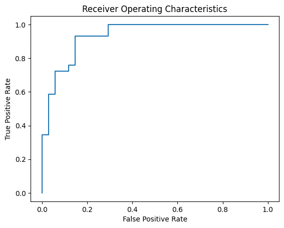
Complete Code
Putting everything together, the following is the complete code of the above
|
1 2 3 4 5 6 7 8 9 10 11 12 13 14 15 16 17 18 19 20 21 22 23 24 25 26 27 28 29 30 31 32 33 34 35 36 37 38 39 40 41 42 43 44 45 46 47 48 49 50 51 52 53 54 55 56 57 58 59 60 61 62 63 64 65 66 67 68 69 70 71 72 73 74 75 76 77 78 79 80 81 82 83 84 85 86 87 88 89 90 91 92 93 94 95 96 97 98 99 100 101 102 103 104 105 106 107 108 109 110 111 112 113 114 115 116 117 118 119 120 121 122 123 124 125 126 127 128 129 130 131 132 133 134 135 136 137 138 139 140 141 142 143 144 145 146 147 148 149 150 151 152 153 154 155 156 157 158 159 160 161 162 163 164 165 166 167 |
import copy import matplotlib.pyplot as plt import numpy as np import pandas as pd import torch import torch.nn as nn import torch.optim as optim 最后,您可以使用 matplotlib 绘制每个 epoch 的损失和准确率,如下所示: from sklearn.metrics import roc_curve from sklearn.model_selection import StratifiedKFold, train_test_split 从 sklearn.preprocessing 导入 LabelEncoder # 读取数据 data = pd.read_csv("sonar.csv", header=None) X = data.iloc[:, 0:60] y = data.iloc[:, 60] # Binary encoding of labels 编码器 = LabelEncoder() 编码器。fit(y) y = encoder.transform(y) # 转换为 2D PyTorch 张量 X = torch.tensor(X.values, dtype=torch.float32) y = torch.tensor(y, dtype=torch.float32).reshape(-1, 1) # Define two models class Wide(nn.Module): def __init__(self): super().__init__() self.hidden = nn.Linear(60, 180) self.relu = nn.ReLU() self.output = nn.Linear(180, 1) self.sigmoid = nn.Sigmoid() def forward(self, x): x = self.relu(self.hidden(x)) x = self.sigmoid(self.output(x)) return x class Deep(nn.Module): def __init__(self): super().__init__() self.layer1 = nn.Linear(60, 60) self.act1 = nn.ReLU() self.layer2 = nn.Linear(60, 60) self.act2 = nn.ReLU() self.layer3 = nn.Linear(60, 60) self.act3 = nn.ReLU() self.output = nn.Linear(60, 1) self.sigmoid = nn.Sigmoid() def forward(self, x): x = self.act1(self.layer1(x)) x = self.act2(self.layer2(x)) x = self.act3(self.layer3(x)) x = self.sigmoid(self.output(x)) return x # 比较模型大小 model1 = Wide() model2 = Deep() print(sum([x.reshape(-1).shape[0] for x in model1.parameters()])) # 11161 print(sum([x.reshape(-1).shape[0] for x in model2.parameters()])) # 11041 # Helper function to train one model def model_train(model, X_train, y_train, X_val, y_val): # 损失函数和优化器 loss_fn = nn.BCELoss() # 二元交叉熵 optimizer = optim.Adam(model.parameters(), lr=0.0001) n_epochs = 300 # number of epochs to run batch_size = 10 # 每个批次的大小 batch_start = torch.arange(0, len(X_train), batch_size) # 保存最佳模型 best_acc = - np.inf # 初始化为负无穷 best_weights = None for epoch in range(n_epochs): model.train() with tqdm.tqdm(batch_start, unit="batch", mininterval=0, disable=True) as bar: bar.set_description(f"Epoch {epoch}") for start in bar: # 获取一个批次 X_batch = X_train[start:start+batch_size] y_batch = y_train[start:start+batch_size] # 前向传播 y_pred = model(X_batch) loss = loss_fn(y_pred, y_batch) # 反向传播 optimizer.zero_grad() loss.backward() # 更新权重 optimizer.step() # 显示进度 acc = (y_pred.round() == y_batch).float().mean() bar.set_postfix( loss=float(loss), acc=float(acc) ) # 在每个 epoch 结束时评估准确率 model.eval() y_pred = model(X_val) acc = (y_pred.round() == y_val).float().mean() acc = float(acc) if acc > best_acc: best_acc = acc best_weights = copy.deepcopy(model.state_dict()) # 恢复模型并返回最佳准确率 model.load_state_dict(best_weights) return best_acc # 训练-测试分割:预留测试集用于最终模型评估 X_train, X_test, y_train, y_test = train_test_split(X, y, train_size=0.7, shuffle=True) # 定义 5 折交叉验证测试框架 kfold = StratifiedKFold(n_splits=5, shuffle=True) cv_scores_wide = [] for train, test in kfold.split(X_train, y_train): # 创建模型,训练,并获取准确率 model = Wide() acc = model_train(model, X_train[train], y_train[train], X_train[test], y_train[test]) print("Accuracy (wide): %.2f" % acc) cv_scores_wide.append(acc) cv_scores_deep = [] for train, test in kfold.split(X_train, y_train): # 创建模型,训练,并获取准确率 model = Deep() acc = model_train(model, X_train[train], y_train[train], X_train[test], y_train[test]) print("Accuracy (deep): %.2f" % acc) cv_scores_deep.append(acc) # 评估模型 wide_acc = np.mean(cv_scores_wide) wide_std = np.std(cv_scores_wide) deep_acc = np.mean(cv_scores_deep) deep_std = np.std(cv_scores_deep) print("Wide: %.2f%% (+/- %.2f%%)" % (wide_acc*100, wide_std*100)) print("Deep: %.2f%% (+/- %.2f%%)" % (deep_acc*100, deep_std*100)) # rebuild model with full set of training data if wide_acc > deep_acc: print("Retrain a wide model") model = Wide() else: print("Retrain a deep model") model = Deep() acc = model_train(model, X_train, y_train, X_test, y_test) print(f"Final model accuracy: {acc*100:.2f}%") model.eval() with torch.no_grad(): # 测试 5 个样本的推理 for i in range(5): y_pred = model(X_test[i:i+1]) print(f"{X_test[i].numpy()} -> {y_pred[0].numpy()} (expected {y_test[i].numpy()})") # Plot the ROC curve y_pred = model(X_test) fpr, tpr, thresholds = roc_curve(y_test, y_pred) plt.plot(fpr, tpr) # ROC curve = TPR vs FPR plt.title("Receiver Operating Characteristics") plt.xlabel("False Positive Rate") plt.ylabel("True Positive Rate") plt.show() |
总结
In this post, you discovered the use of PyTorch to build a binary classification model.
You learned how you can work through a binary classification problem step-by-step with PyTorch, specifically
- How to load and prepare data for use in PyTorch
- How to create neural network models and use k-fold cross validation to compare them
- How to train a binary classification model and obtain the receiver operating characteristics curve for it
开始使用PyTorch进行深度学习!
学习如何构建深度学习模型
...使用新发布的PyTorch 2.0库
在我的新电子书中探索如何实现
使用 PyTorch进行深度学习
它提供了包含数百个可用代码的自学教程,让你从新手变成专家。它将使你掌握:
张量操作、训练、评估、超参数优化等等...


Hello, there is a problem I don’t understand. In the two loops of fold.split, there is model=Wide() or Deep() at the beginning of each loop. Is this a reset of the model? If each loop continues to train the best model in the previous cycle, Whether model=Wide() or Deep() should be placed outside the loop to avoid reassignment of the model