逻辑回归是一种预测事件发生概率的回归类型。它用于分类问题,并在机器学习、人工智能和数据挖掘领域有许多应用。
逻辑回归的公式是对线性函数应用 sigmoid 函数。本文将讨论如何构建一个逻辑回归分类器。虽然之前您一直在处理单变量数据集,但在这里我们将使用流行的 MNIST 数据集来训练和测试我们的模型。读完本文,您将学到:
- 如何在 PyTorch 中使用逻辑回归及其在现实问题中的应用。
- 如何加载和分析 torchvision 数据集。
- 如何在图像数据集上构建和训练逻辑回归分类器。
通过我的《用PyTorch进行深度学习》一书来启动你的项目。它提供了包含可用代码的自学教程。
让我们开始吧。

在 PyTorch 中构建逻辑回归分类器。
图片来源:Catgirlmutant。部分权利保留。
概述
本教程分为四个部分;它们是:
- MNIST 数据集
- 将数据集加载到 DataLoader 中
- 使用
nn.Module构建模型 - 训练分类器
MNIST 数据集
您将使用 MNIST 数据集训练和测试逻辑回归模型。该数据集包含 60,000 张用于训练的图像和 10,000 张用于测试样本外性能的图像。
MNIST 数据集非常流行,以至于它是 PyTorch 的一部分。以下是如何在 PyTorch 中加载 MNIST 数据集的训练和测试样本。
|
1 2 3 4 5 6 7 8 9 10 11 12 13 |
import torch import torchvision.transforms as transforms from torchvision import datasets # 加载训练数据 train_dataset = datasets.MNIST(root='./data', train=True, transform=transforms.ToTensor(), download=True) #加载测试数据 test_dataset = datasets.MNIST(root='./data', train=False, transform=transforms.ToTensor()) |
数据集将按如下方式下载并提取到目录中。
|
1 2 3 4 5 6 7 8 9 10 11 12 13 14 15 16 17 18 19 |
Downloading http://yann.lecun.com/exdb/mnist/train-images-idx3-ubyte.gz Downloading http://yann.lecun.com/exdb/mnist/train-images-idx3-ubyte.gz to ./data/MNIST/raw/train-images-idx3-ubyte.gz 0%| | 0/9912422 [00:00<?, ?it/s] Extracting ./data/MNIST/raw/train-images-idx3-ubyte.gz to ./data/MNIST/raw Downloading http://yann.lecun.com/exdb/mnist/train-labels-idx1-ubyte.gz Downloading http://yann.lecun.com/exdb/mnist/train-labels-idx1-ubyte.gz to ./data/MNIST/raw/train-labels-idx1-ubyte.gz 0%| | 0/28881 [00:00<?, ?it/s] Extracting ./data/MNIST/raw/train-labels-idx1-ubyte.gz to ./data/MNIST/raw Downloading http://yann.lecun.com/exdb/mnist/t10k-images-idx3-ubyte.gz Downloading http://yann.lecun.com/exdb/mnist/t10k-images-idx3-ubyte.gz to ./data/MNIST/raw/t10k-images-idx3-ubyte.gz 0%| | 0/1648877 [00:00<?, ?it/s] Extracting ./data/MNIST/raw/t10k-images-idx3-ubyte.gz to ./data/MNIST/raw Downloading http://yann.lecun.com/exdb/mnist/t10k-labels-idx1-ubyte.gz Downloading http://yann.lecun.com/exdb/mnist/t10k-labels-idx1-ubyte.gz to ./data/MNIST/raw/t10k-labels-idx1-ubyte.gz 0%| | 0/4542 [00:00<?, ?it/s] Extracting ./data/MNIST/raw/t10k-labels-idx1-ubyte.gz to ./data/MNIST/raw |
让我们验证一下数据集中训练和测试样本的数量。
|
1 2 |
print("number of training samples: " + str(len(train_dataset)) + "\n" + "number of testing samples: " + str(len(test_dataset))) |
输出结果为:
|
1 2 |
number of training samples: 60000 number of testing samples: 10000 |
数据集中的每个样本都是一个图像和标签的对。要检查训练数据第一个元素的数据类型和大小,您可以使用 type() 和 size() 方法。
|
1 2 |
print("datatype of the 1st training sample: ", train_dataset[0][0].type()) print("size of the 1st training sample: ", train_dataset[0][0].size()) |
输出如下:
|
1 2 |
datatype of the 1st training sample: torch.FloatTensor size of the 1st training sample: torch.Size([1, 28, 28]) |
您可以通过列表索引访问数据集中的样本。数据集中的第一个样本是一个 FloatTensor,它是一个 $28\times 28$ 像素的灰度图像(即一个通道),因此大小为 [1, 28, 28]。
现在,让我们检查训练集中前两个样本的标签。
|
1 2 3 |
# 检查第一个训练样本的标签 print("label of the first taining sample: ", train_dataset[0][1]) print("label of the second taining sample: ", train_dataset[1][1]) |
这表明:
|
1 2 |
label of the first taining sample: 5 label of the second taining sample: 0 |
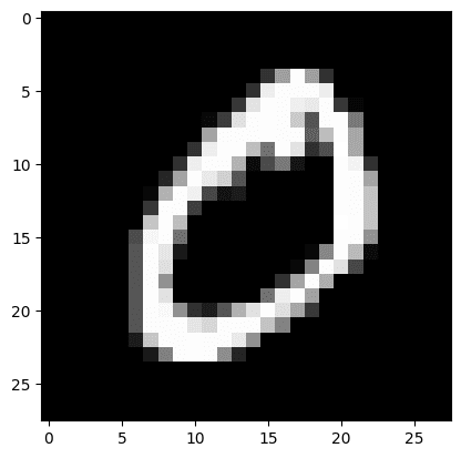
从上面的输出可以看出,训练集中的前两个图像分别代表数字“5”和“0”。让我们显示这两张图像以确认。
|
1 2 3 4 5 6 |
img_5 = train_dataset[0][0].numpy().reshape(28, 28) plt.imshow(img_5, cmap='gray') plt.show() img_0 = train_dataset[1][0].numpy().reshape(28, 28) plt.imshow(img_0, cmap='gray') plt.show() |
您应该会看到这两个数字:
将数据集加载到 DataLoader 中
通常,您不会直接在训练中使用数据集,而是通过 DataLoader 类。这允许您按批次读取数据,而不是按样本读取。
在下面,数据将以 32 的批次大小加载到 DataLoader 中。
|
1 2 3 4 5 6 7 |
... from torch.utils.data import DataLoader # 将训练和测试数据样本加载到 dataloader 中 batach_size = 32 train_loader = DataLoader(dataset=train_dataset, batch_size=batach_size, shuffle=True) test_loader = DataLoader(dataset=test_dataset, batch_size=batach_size, shuffle=False) |
想开始构建带有注意力的 Transformer 模型吗?
立即参加我的免费12天电子邮件速成课程(含示例代码)。
点击注册,同时获得该课程的免费PDF电子书版本。
使用 nn.Module 构建模型
我们将为逻辑回归模型使用 nn.Module 来构建模型类。此类与之前的帖子中的类似,但输入和输出的数量是可配置的。
|
1 2 3 4 5 6 7 8 9 10 |
# 为逻辑回归构建自定义模块 class LogisticRegression(torch.nn.Module): # 构建构造函数 def __init__(self, n_inputs, n_outputs): super(LogisticRegression, self).__init__() self.linear = torch.nn.Linear(n_inputs, n_outputs) # 进行预测 def forward(self, x): y_pred = torch.sigmoid(self.linear(x)) return y_pred |
此模型将接受 $28\times 28$ 像素的手写数字图像作为输入,并将其分类到 0 到 9 的 10 个输出类别之一。因此,以下是实例化模型的方法。
|
1 2 3 4 |
# 实例化模型 n_inputs = 28*28 # 形成一个 784 的一维向量 n_outputs = 10 log_regr = LogisticRegression(n_inputs, n_outputs) |
训练分类器
您将使用随机梯度下降作为优化器,学习率为 0.001,交叉熵作为损失度量来训练此模型。
然后,模型将训练 50 个 epoch。请注意,您使用了 view() 方法将图像矩阵展平成行,以匹配逻辑回归模型输入的形状。
|
1 2 3 4 5 6 7 8 9 10 11 12 13 14 15 16 17 18 19 20 21 22 23 24 25 26 27 |
... # 定义优化器 optimizer = torch.optim.SGD(log_regr.parameters(), lr=0.001) # 定义交叉熵损失 criterion = torch.nn.CrossEntropyLoss() epochs = 50 Loss = [] acc = [] for epoch in range(epochs): for i, (images, labels) in enumerate(train_loader): optimizer.zero_grad() outputs = log_regr(images.view(-1, 28*28)) loss = criterion(outputs, labels) # Loss.append(loss.item()) loss.backward() optimizer.step() Loss.append(loss.item()) correct = 0 for images, labels in test_loader: outputs = log_regr(images.view(-1, 28*28)) _, predicted = torch.max(outputs.data, 1) correct += (predicted == labels).sum() accuracy = 100 * (correct.item()) / len(test_dataset) acc.append(accuracy) print('Epoch: {}. Loss: {}. Accuracy: {}'.format(epoch, loss.item(), accuracy)) |
在训练过程中,您应该会看到如下进度:
|
1 2 3 4 5 6 7 8 9 10 11 12 |
Epoch: 0. Loss: 2.211054563522339. Accuracy: 61.63 Epoch: 1. Loss: 2.1178536415100098. Accuracy: 74.81 Epoch: 2. Loss: 2.0735440254211426. Accuracy: 78.47 Epoch: 3. Loss: 2.040225028991699. Accuracy: 80.17 Epoch: 4. Loss: 1.9637292623519897. Accuracy: 81.05 Epoch: 5. Loss: 2.000900983810425. Accuracy: 81.44 ... Epoch: 45. Loss: 1.6549798250198364. Accuracy: 86.3 Epoch: 46. Loss: 1.7053509950637817. Accuracy: 86.31 Epoch: 47. Loss: 1.7396119832992554. Accuracy: 86.36 Epoch: 48. Loss: 1.6963073015213013. Accuracy: 86.37 Epoch: 49. Loss: 1.6838685274124146. Accuracy: 86.46 |
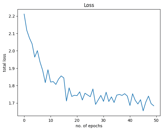
仅训练 50 个 epoch 就达到了大约 86% 的准确率。如果模型训练时间更长,准确率还可以进一步提高。
让我们可视化损失和准确率图表。以下是损失图:
|
1 2 3 4 5 |
plt.plot(Loss) plt.xlabel("no. of epochs") plt.ylabel("总损失") plt.title("Loss") plt.show() |
这是准确率图:
|
1 2 3 4 5 |
plt.plot(acc) plt.xlabel("no. of epochs") plt.ylabel("total accuracy") plt.title("Accuracy") plt.show() |

把所有东西放在一起,下面是完整的代码。
|
1 2 3 4 5 6 7 8 9 10 11 12 13 14 15 16 17 18 19 20 21 22 23 24 25 26 27 28 29 30 31 32 33 34 35 36 37 38 39 40 41 42 43 44 45 46 47 48 49 50 51 52 53 54 55 56 57 58 59 60 61 62 63 64 65 66 67 68 69 70 71 72 73 74 75 76 77 78 79 80 81 82 83 84 85 86 87 88 89 90 |
import torch import torchvision.transforms as transforms from torchvision import datasets from torch.utils.data import DataLoader import matplotlib.pyplot as plt # 加载训练数据 train_dataset = datasets.MNIST(root='./data', train=True, transform=transforms.ToTensor(), download=True) # 加载测试数据 test_dataset = datasets.MNIST(root='./data', train=False, transform=transforms.ToTensor()) print("number of training samples: " + str(len(train_dataset)) + "\n" + "number of testing samples: " + str(len(test_dataset))) print("datatype of the 1st training sample: ", train_dataset[0][0].type()) print("size of the 1st training sample: ", train_dataset[0][0].size()) # 检查第一个训练样本的标签 print("label of the first taining sample: ", train_dataset[0][1]) print("label of the second taining sample: ", train_dataset[1][1]) img_5 = train_dataset[0][0].numpy().reshape(28, 28) plt.imshow(img_5, cmap='gray') plt.show() img_0 = train_dataset[1][0].numpy().reshape(28, 28) plt.imshow(img_0, cmap='gray') plt.show() # 将训练和测试数据样本加载到 dataloader 中 batach_size = 32 train_loader = DataLoader(dataset=train_dataset, batch_size=batach_size, shuffle=True) test_loader = DataLoader(dataset=test_dataset, batch_size=batach_size, shuffle=False) # 为逻辑回归构建自定义模块 class LogisticRegression(torch.nn.Module): # 构建构造函数 def __init__(self, n_inputs, n_outputs): super().__init__() self.linear = torch.nn.Linear(n_inputs, n_outputs) # 进行预测 def forward(self, x): y_pred = torch.sigmoid(self.linear(x)) return y_pred # 实例化模型 n_inputs = 28*28 # 形成一个 784 的一维向量 n_outputs = 10 log_regr = LogisticRegression(n_inputs, n_outputs) # 定义优化器 optimizer = torch.optim.SGD(log_regr.parameters(), lr=0.001) # 定义交叉熵损失 criterion = torch.nn.CrossEntropyLoss() epochs = 50 Loss = [] acc = [] for epoch in range(epochs): for i, (images, labels) in enumerate(train_loader): optimizer.zero_grad() outputs = log_regr(images.view(-1, 28*28)) loss = criterion(outputs, labels) # Loss.append(loss.item()) loss.backward() optimizer.step() Loss.append(loss.item()) correct = 0 for images, labels in test_loader: outputs = log_regr(images.view(-1, 28*28)) _, predicted = torch.max(outputs.data, 1) correct += (predicted == labels).sum() accuracy = 100 * (correct.item()) / len(test_dataset) acc.append(accuracy) print('Epoch: {}. Loss: {}. Accuracy: {}'.format(epoch, loss.item(), accuracy)) plt.plot(Loss) plt.xlabel("no. of epochs") plt.ylabel("总损失") plt.title("Loss") plt.show() plt.plot(acc) plt.xlabel("no. of epochs") plt.ylabel("total accuracy") plt.title("Accuracy") plt.show() |
总结
在本教程中,您学习了如何在 PyTorch 中构建一个多类逻辑回归分类器。具体来说,您学习了:
- 如何在 PyTorch 中使用逻辑回归及其在现实问题中的应用。
- 如何加载和分析 torchvision 数据集。
- 如何在图像数据集上构建和训练逻辑回归分类器。
开始使用PyTorch进行深度学习!
学习如何构建深度学习模型
...使用新发布的PyTorch 2.0库
在我的新电子书中探索如何实现
使用 PyTorch进行深度学习
它提供了包含数百个可用代码的自学教程,让你从新手变成专家。它将使你掌握:
张量操作、训练、评估、超参数优化等等...


感谢您提供的精彩教程!
非常欢迎 Eduardo!我们感谢您的反馈和支持。
教程很棒,也非常有指导意义,谢谢!
但是我有一个问题。教程中使用了 Torch CrossEntropyLoss,它内部包含了一个 softmax 步骤。所以,这更像是一个 softmax 分类(适用于多类)的例子,而不是逻辑回归(适用于二分类)的例子。
事实上,如果我在 forward 函数中移除 sigmoid 步骤,我的准确率会更高。
我刚进入这个领域,您能评论一下吗?
你好 Alberto…你说得对!二分类是多分类的一个子集,所以你的结果是有道理的。
我认为这个实现是错误的。
应该移除 sigmoids,并用 BCEWithLogitsLoss 替换 CrossEntropyLoss。
事实上,CrossEntropyLoss 内部应用了 softmax,而 BCEWithLogitsLoss 内部应用了 sigmoid。
你好 Marco…谢谢你的反馈!你能否提供更多关于你获得的结果的细节,以证实这个实现是错误的?
嗨 James,
如果你查看 CrossEntropyLoss 的 pydoc(https://pytorch.ac.cn/docs/stable/generated/torch.nn.CrossEntropyLoss.html),你会看到它期望的输入是每个类的未归一化 logits。所以,基本上,在一个简单的单层密集网络中,它应该是线性层的输出。而在你的例子中,输入是 sigmoid 的输出。最后一个步骤是不需要的,因为它已经被 CrossEntropyLoss 应用了。你的例子实际上是 y = loss(softmax(sigmoid(x)))。
我完全同意 Marco F 的评论。该模型目前是不正确的。
为了好玩,我在 IRIS 数据集上试了一下,并将其与 sklearn 的逻辑回归进行了比较。
当你从模型中移除 sigmoid 部分时,你得到与 sklearn 库相同的损失。但是,使用 sigmoid 函数你会得到不同的(而且实际上非常糟糕的)结果。
谢谢你的反馈 Clemens!
既然多个评论者都指出了错误,为什么这个还在呢?