进化策略是一种随机全局优化算法。
它是一种进化算法,与其他算法(如遗传算法)相关,但它是专门为连续函数优化而设计的。
在本教程中,您将学习如何实现进化策略优化算法。
完成本教程后,您将了解:
- 进化策略是一种随机全局优化算法,其灵感来自于自然选择的生物进化理论。
- 进化策略有标准术语,并且算法有两种常见版本,分别称为 (mu, lambda)-ES 和 (mu + lambda)-ES。
- 如何实现进化策略算法并将其应用于连续目标函数。
开始您的项目,阅读我的新书《机器学习优化》,其中包含分步教程和所有示例的Python源代码文件。
让我们开始吧。
在 Python 中从零开始实现进化策略
照片由 Alexis A. Bermúdez 拍摄,保留部分权利。
教程概述
本教程分为三个部分;它们是:
- 进化策略
- 开发 (mu, lambda)-ES
- 开发 (mu + lambda)-ES
进化策略
进化策略,有时也称为进化策略(单数)或 ES,是一种随机全局优化算法。
该技术于 20 世纪 60 年代开发,供工程师手动实现,用于风洞中的最小阻力设计。
进化策略 (ES) 系列算法由 Ingo Rechenberg 和 Hans-Paul Schwefel 于 20 世纪 60 年代中期在柏林工业大学开发。
— 第 31 页,元启发式算法要点,2011 年。
进化策略是一种进化算法,其灵感来自自然选择的生物进化理论。与其他进化算法不同,它不使用任何形式的交叉;相反,候选解的修改仅限于变异算子。通过这种方式,进化策略可以被认为是并行随机爬山的一种类型。
该算法涉及一个候选解的种群,最初是随机生成的。算法的每次迭代首先评估解的种群,然后删除除了一部分最优解之外的所有解,这称为截断选择。剩余的解(父代)中的每一个都用作生成若干新候选解(变异)的基础,这些新候选解会替换父代或与父代竞争种群中的位置,以便在算法的下一次迭代(代)中进行考虑。
此过程有多种变体,并且有标准术语来总结算法。种群大小称为lambda,每次迭代选择的父代数量称为mu。
每个父代创建的子代数量计算为 (lambda / mu),应选择参数使除法无余数。
- mu:每次迭代选择的父代数量。
- lambda:种群大小。
- lambda / mu:每个选定父代生成的子代数量。
使用括号表示法描述算法配置,例如(mu, lambda)-ES。例如,如果mu=5且lambda=20,则将其总结为(5, 20)-ES。mu和lambda参数之间的逗号 (,) 表示子代在算法的每次迭代中直接替换父代。
- (mu, lambda)-ES:一种进化策略版本,其中子代替换父代。
mu和lambda参数的加号 (+) 分隔表示子代和父代将共同定义下一迭代的种群。
- (mu + lambda)-ES:一种进化策略版本,其中子代和父代被添加到种群中。
随机爬山算法可以实现为进化策略,并且表示法为(1 + 1)-ES。
这是模拟或规范的 ES 算法,文献中有许多扩展和变体。
现在我们熟悉了进化策略,就可以探索如何实现该算法了。
想要开始学习优化算法吗?
立即参加我为期7天的免费电子邮件速成课程(附示例代码)。
点击注册,同时获得该课程的免费PDF电子书版本。
开发 (mu, lambda)-ES
在本节中,我们将开发一个(mu, lambda)-ES,即一种子代替换父代的算法版本。
首先,让我们定义一个具有挑战性的优化问题作为实现算法的基础。
Ackley 函数是多模态目标函数的一个示例,它具有单个全局最优解和多个局部最优解,局部搜索可能会陷入其中。
因此,需要一种全局优化技术。它是一个二维目标函数,在 [0,0] 处有全局最优解,其值为 0.0。
下面的例子实现了 Ackley 函数并创建了一个三维曲面图,显示了全局最优解和多个局部最优解。
|
1 2 3 4 5 6 7 8 9 10 11 12 13 14 15 16 17 18 19 20 21 22 23 24 25 26 27 28 29 30 |
# ackley 多峰函数 from numpy import arange from numpy import exp from numpy import sqrt from numpy import cos from numpy import e from numpy import pi from numpy import meshgrid from matplotlib import pyplot from mpl_toolkits.mplot3d import Axes3D # 目标函数 def objective(x, y): return -20.0 * exp(-0.2 * sqrt(0.5 * (x**2 + y**2))) - exp(0.5 * (cos(2 * pi * x) + cos(2 * pi * y))) + e + 20 # 定义输入范围 r_min, r_max = -5.0, 5.0 # 以 0.1 为增量均匀采样输入范围 xaxis = arange(r_min, r_max, 0.1) yaxis = arange(r_min, r_max, 0.1) # 从坐标轴创建网格 x, y = meshgrid(xaxis, yaxis) # 计算目标值 results = objective(x, y) # 使用 jet 配色方案创建曲面图 figure = pyplot.figure() axis = figure.gca(projection='3d') axis.plot_surface(x, y, results, cmap='jet') # 显示绘图 pyplot.show() |
运行该示例会创建 Ackley 函数的曲面图,显示大量的局部最优解。
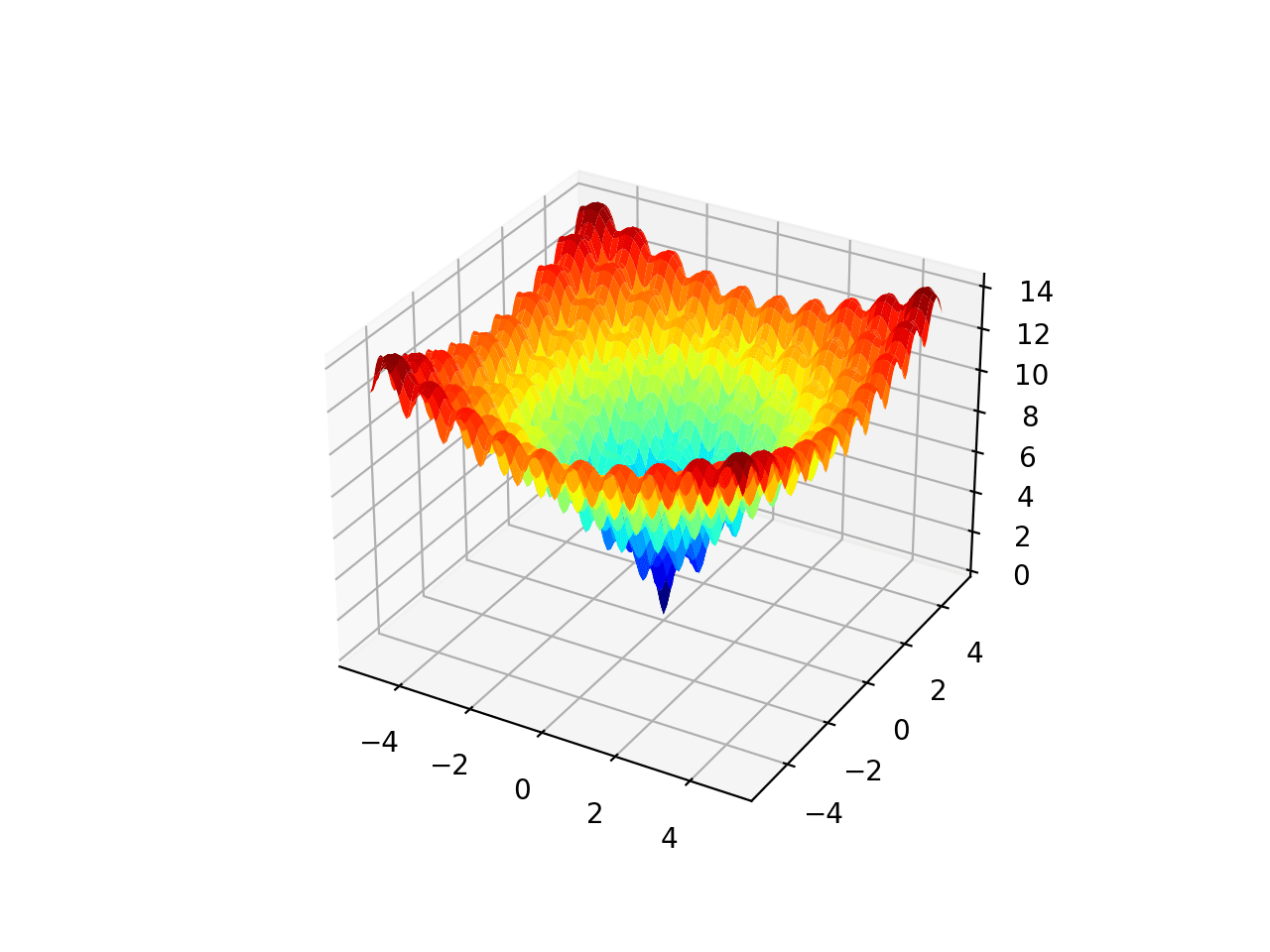
Ackley 多峰函数的三维曲面图
我们将生成随机候选解以及现有候选解的修改版本。所有候选解都必须在搜索问题的边界内,这一点很重要。
为了实现这一点,我们将开发一个函数来检查候选解是否在搜索边界内,如果不在,则将其丢弃并生成另一个解。
下面的 `in_bounds()` 函数将接收一个候选解(点)和搜索空间边界的定义(bounds),如果解在搜索边界内,则返回 True,否则返回 False。
|
1 2 3 4 5 6 7 8 |
# 检查一个点是否在搜索范围内 def in_bounds(point, bounds): # 枚举点的所有维度 for d in range(len(bounds)): # 检查此维度是否超出界限 if point[d] < bounds[d, 0] or point[d] > bounds[d, 1]: return False return True |
然后,我们可以在生成“lam”(例如,lambda)个随机候选解的初始种群时使用此函数。
例如
|
1 2 3 4 5 6 7 8 |
... # 初始种群 population = list() for _ in range(lam): candidate = None while candidate is None or not in_bounds(candidate, bounds): candidate = bounds[:, 0] + rand(len(bounds)) * (bounds[:, 1] - bounds[:, 0]) population.append(candidate) |
接下来,我们可以迭代固定次数的算法。每次迭代首先评估种群中的每个候选解。
我们将计算得分并将它们存储在一个单独的并行列表中。
|
1 2 3 |
... # 评估种群的适应度 scores = [objective(c) for c in population] |
接下来,我们需要选择得分最高的“mu”个父代,在本例中是得分最低的,因为我们在最小化目标函数。
我们将分两步进行。首先,我们将根据得分按升序对候选解进行排名,以便得分最低的解排名为 0,下一个排名为 1,依此类推。我们可以通过双重调用 argsort 函数 来实现此目的。
然后,我们将使用排名并选择排名低于“mu”值的父代。这意味着如果 `mu` 设置为 5 以选择 5 个父代,则只选择排名在 0 到 4 之间的父代。
|
1 2 3 4 5 |
... # 按升序排列得分 ranks = argsort(argsort(scores)) # 选择排名前 mu 的解的索引 selected = [i for i,_ in enumerate(ranks) if ranks[i] < mu] |
然后,我们可以为每个选定的父代创建子代。
首先,我们必须计算每个父代要创建的子代总数。
|
1 2 3 |
... # 计算每个父代的子代数量 n_children = int(lam / mu) |
然后,我们可以遍历每个父代并创建它们的修改版本。
我们将使用一种类似于随机爬山的技术来创建子代。具体来说,每个变量将使用以当前值为均值、标准差提供为“步长”超参数的高斯分布进行采样。
|
1 2 3 4 5 6 |
... # 为父代创建子代 for _ in range(n_children): child = None while child is None or not in_bounds(child, bounds): child = population[i] + randn(len(bounds)) * step_size |
我们还可以检查每个选定的父代是否优于迄今为止看到的最佳解,以便我们可以在搜索结束时返回最佳解。
|
1 2 3 4 5 |
... # 检查此父代是否为迄今为止见过的最佳解 if scores[i] < best_eval: best, best_eval = population[i], scores[i] print('%d, Best: f(%s) = %.5f' % (epoch, best, best_eval)) |
创建的子代可以添加到列表中,并在算法迭代结束时用子代列表替换种群。
|
1 2 3 |
... # 用子代替换种群 population = children |
我们可以将所有这些整合到一个名为 `es_comma()` 的函数中,该函数执行进化策略算法的逗号版本。
该函数采用目标函数的名称、搜索空间的边界、迭代次数、步长以及 mu 和 lambda 超参数,并返回搜索过程中找到的最佳解及其评估值。
|
1 2 3 4 5 6 7 8 9 10 11 12 13 14 15 16 17 18 19 20 21 22 23 24 25 26 27 28 29 30 31 32 33 34 35 36 |
# 进化策略 (mu, lambda) 算法 def es_comma(objective, bounds, n_iter, step_size, mu, lam): best, best_eval = None, 1e+10 # 计算每个父代的子代数量 n_children = int(lam / mu) # 初始种群 population = list() for _ in range(lam): candidate = None while candidate is None or not in_bounds(candidate, bounds): candidate = bounds[:, 0] + rand(len(bounds)) * (bounds[:, 1] - bounds[:, 0]) population.append(candidate) # 执行搜索 for epoch in range(n_iter): # 评估种群的适应度 scores = [objective(c) for c in population] # 按升序排列得分 ranks = argsort(argsort(scores)) # 选择排名前 mu 的解的索引 selected = [i for i,_ in enumerate(ranks) if ranks[i] < mu] # 从父代创建子代 children = list() for i in selected: # 检查此父代是否为迄今为止见过的最佳解 if scores[i] < best_eval: best, best_eval = population[i], scores[i] print('%d, Best: f(%s) = %.5f' % (epoch, best, best_eval)) # 为父代创建子代 for _ in range(n_children): child = None while child is None or not in_bounds(child, bounds): child = population[i] + randn(len(bounds)) * step_size children.append(child) # 用子代替换种群 population = children return [best, best_eval] |
接下来,我们可以将此算法应用于我们的 Ackley 目标函数。
我们将运行算法 5,000 次迭代,并在搜索空间中使用 0.15 的步长。我们将使用 100 的种群大小(lambda),选择 20 个父代(mu)。这些超参数是在经过一些试错后选择的。
在搜索结束时,我们将报告搜索过程中找到的最佳候选解。
|
1 2 3 4 5 6 7 8 9 10 11 12 13 14 15 16 17 |
... # 播种伪随机数生成器 seed(1) # 定义输入范围 bounds = asarray([[-5.0, 5.0], [-5.0, 5.0]]) # 定义总迭代次数 n_iter = 5000 # 定义最大步长 step_size = 0.15 # 选择的父代数量 mu = 20 # 父代生成的子代数量 lam = 100 # 执行进化策略 (mu, lambda) 搜索 best, score = es_comma(objective, bounds, n_iter, step_size, mu, lam) print('Done!') print('f(%s) = %f' % (best, score)) |
将所有内容整合在一起,下面列出了将逗号版本的进化策略算法应用于 Ackley 目标函数的完整示例。
|
1 2 3 4 5 6 7 8 9 10 11 12 13 14 15 16 17 18 19 20 21 22 23 24 25 26 27 28 29 30 31 32 33 34 35 36 37 38 39 40 41 42 43 44 45 46 47 48 49 50 51 52 53 54 55 56 57 58 59 60 61 62 63 64 65 66 67 68 69 70 71 72 73 74 75 76 77 78 79 80 |
# Ackley 目标函数的进化策略 (mu, lambda) from numpy import asarray from numpy import exp from numpy import sqrt from numpy import cos from numpy import e from numpy import pi from numpy import argsort from numpy.random import randn from numpy.random import rand from numpy.random import seed # 目标函数 def objective(v): x, y = v return -20.0 * exp(-0.2 * sqrt(0.5 * (x**2 + y**2))) - exp(0.5 * (cos(2 * pi * x) + cos(2 * pi * y))) + e + 20 # 检查一个点是否在搜索范围内 def in_bounds(point, bounds): # 枚举点的所有维度 for d in range(len(bounds)): # 检查此维度是否超出界限 if point[d] < bounds[d, 0] or point[d] > bounds[d, 1]: return False return True # 进化策略 (mu, lambda) 算法 def es_comma(objective, bounds, n_iter, step_size, mu, lam): best, best_eval = None, 1e+10 # 计算每个父代的子代数量 n_children = int(lam / mu) # 初始种群 population = list() for _ in range(lam): candidate = None while candidate is None or not in_bounds(candidate, bounds): candidate = bounds[:, 0] + rand(len(bounds)) * (bounds[:, 1] - bounds[:, 0]) population.append(candidate) # 执行搜索 for epoch in range(n_iter): # 评估种群的适应度 scores = [objective(c) for c in population] # 按升序排列得分 ranks = argsort(argsort(scores)) # 选择排名前 mu 的解的索引 selected = [i for i,_ in enumerate(ranks) if ranks[i] < mu] # 从父代创建子代 children = list() for i in selected: # 检查此父代是否为迄今为止见过的最佳解 if scores[i] < best_eval: best, best_eval = population[i], scores[i] print('%d, Best: f(%s) = %.5f' % (epoch, best, best_eval)) # 为父代创建子代 for _ in range(n_children): child = None while child is None or not in_bounds(child, bounds): child = population[i] + randn(len(bounds)) * step_size children.append(child) # 用子代替换种群 population = children return [best, best_eval] # 播种伪随机数生成器 seed(1) # 定义输入范围 bounds = asarray([[-5.0, 5.0], [-5.0, 5.0]]) # 定义总迭代次数 n_iter = 5000 # 定义最大步长 step_size = 0.15 # 选择的父代数量 mu = 20 # 父代生成的子代数量 lam = 100 # 执行进化策略 (mu, lambda) 搜索 best, score = es_comma(objective, bounds, n_iter, step_size, mu, lam) print('Done!') print('f(%s) = %f' % (best, score)) |
运行示例会在每次找到更好的解时报告候选解和得分,然后在搜索结束时报告找到的最佳解。
注意:由于算法或评估过程的随机性,或数值精度的差异,您的结果可能会有所不同。请考虑运行示例几次并比较平均结果。
在这种情况下,我们可以看到在搜索过程中性能提高了约 22 次,并且最佳解决方案接近最优值。
毫无疑问,该解决方案可以作为局部搜索算法的起点,以进行进一步的改进,这是在使用 ES 等全局优化算法时的常见做法。
|
1 2 3 4 5 6 7 8 9 10 11 12 13 14 15 16 17 18 19 20 21 22 23 24 |
0, 最佳: f([-0.82977995 2.20324493]) = 6.91249 0, 最佳: f([-1.03232526 0.38816734]) = 4.49240 1, 最佳: f([-1.02971385 0.21986453]) = 3.68954 2, 最佳: f([-0.98361735 0.19391181]) = 3.40796 2, 最佳: f([-0.98189724 0.17665892]) = 3.29747 2, 最佳: f([-0.07254927 0.67931431]) = 3.29641 3, 最佳: f([-0.78716147 0.02066442]) = 2.98279 3, 最佳: f([-1.01026218 -0.03265665]) = 2.69516 3, 最佳: f([-0.08851828 0.26066485]) = 2.00325 4, 最佳: f([-0.23270782 0.04191618]) = 1.66518 4, 最佳: f([-0.01436704 0.03653578]) = 0.15161 7, 最佳: f([0.01247004 0.01582657]) = 0.06777 9, 最佳: f([0.00368129 0.00889718]) = 0.02970 25, 最佳: f([ 0.00666975 -0.0045051 ]) = 0.02449 33, 最佳: f([-0.00072633 -0.00169092]) = 0.00530 211, 最佳: f([2.05200123e-05 1.51343187e-03]) = 0.00434 315, 最佳: f([ 0.00113528 -0.00096415]) = 0.00427 418, 最佳: f([ 0.00113735 -0.00030554]) = 0.00337 491, 最佳: f([ 0.00048582 -0.00059587]) = 0.00219 704, 最佳: f([-6.91643854e-04 -4.51583644e-05]) = 0.00197 1504, 最佳: f([ 2.83063223e-05 -4.60893027e-04]) = 0.00131 3725, 最佳: f([ 0.00032757 -0.00023643]) = 0.00115 完成! f([ 0.00032757 -0.00023643]) = 0.001147 |
现在我们已经熟悉了如何实现进化策略的逗号版本,让我们看看如何实现加号版本。
开发 (mu + lambda)-ES
进化策略算法的加号版本与逗号版本非常相似。
主要区别在于,最后,子代和父代共同构成种群,而不是仅仅子代。这使得父代能够与子代竞争下一迭代的选择。
这可能导致搜索算法的行为更加贪婪,并可能过早收敛到局部最优值(次优解)。这样做的好处是算法能够利用找到的优秀候选解,并专注于该区域的候选解,从而可能找到进一步的改进。
我们可以通过修改函数以在创建子代时添加父代来实现该算法的加号版本。
|
1 2 3 |
... # 保留父代 children.append(population[i]) |
更新后的函数版本增加了此功能,并有一个新名称 *es_plus()*,如下所示。
|
1 2 3 4 5 6 7 8 9 10 11 12 13 14 15 16 17 18 19 20 21 22 23 24 25 26 27 28 29 30 31 32 33 34 35 36 37 38 |
# 进化策略 (mu + lambda) 算法 def es_plus(objective, bounds, n_iter, step_size, mu, lam): best, best_eval = None, 1e+10 # 计算每个父代的子代数量 n_children = int(lam / mu) # 初始种群 population = list() for _ in range(lam): candidate = None while candidate is None or not in_bounds(candidate, bounds): candidate = bounds[:, 0] + rand(len(bounds)) * (bounds[:, 1] - bounds[:, 0]) population.append(candidate) # 执行搜索 for epoch in range(n_iter): # 评估种群的适应度 scores = [objective(c) for c in population] # 按升序排列得分 ranks = argsort(argsort(scores)) # 选择排名前 mu 的解的索引 selected = [i for i,_ in enumerate(ranks) if ranks[i] < mu] # 从父代创建子代 children = list() for i in selected: # 检查此父代是否为迄今为止见过的最佳解 if scores[i] < best_eval: best, best_eval = population[i], scores[i] print('%d, Best: f(%s) = %.5f' % (epoch, best, best_eval)) # 保留父代 children.append(population[i]) # 为父代创建子代 for _ in range(n_children): child = None while child is None or not in_bounds(child, bounds): child = population[i] + randn(len(bounds)) * step_size children.append(child) # 用子代替换种群 population = children return [best, best_eval] |
我们可以将此版本的算法应用于 Ackley 目标函数,其超参数与上一节中使用的相同。
完整的示例如下所示。
|
1 2 3 4 5 6 7 8 9 10 11 12 13 14 15 16 17 18 19 20 21 22 23 24 25 26 27 28 29 30 31 32 33 34 35 36 37 38 39 40 41 42 43 44 45 46 47 48 49 50 51 52 53 54 55 56 57 58 59 60 61 62 63 64 65 66 67 68 69 70 71 72 73 74 75 76 77 78 79 80 81 |
# Ackley 目标函数的进化策略 (mu + lambda) from numpy import asarray from numpy import exp from numpy import sqrt from numpy import cos from numpy import e from numpy import pi from numpy import argsort from numpy.random import randn from numpy.random import rand from numpy.random import seed # 目标函数 def objective(v): x, y = v return -20.0 * exp(-0.2 * sqrt(0.5 * (x**2 + y**2))) - exp(0.5 * (cos(2 * pi * x) + cos(2 * pi * y))) + e + 20 # 检查一个点是否在搜索范围内 def in_bounds(point, bounds): # 枚举点的所有维度 for d in range(len(bounds)): # 检查此维度是否超出界限 if point[d] < bounds[d, 0] or point[d] > bounds[d, 1]: return False return True # 进化策略 (mu + lambda) 算法 def es_plus(objective, bounds, n_iter, step_size, mu, lam): best, best_eval = None, 1e+10 # 计算每个父代的子代数量 n_children = int(lam / mu) # 初始种群 population = list() for _ in range(lam): candidate = None while candidate is None or not in_bounds(candidate, bounds): candidate = bounds[:, 0] + rand(len(bounds)) * (bounds[:, 1] - bounds[:, 0]) population.append(candidate) # 执行搜索 for epoch in range(n_iter): # 评估种群的适应度 scores = [objective(c) for c in population] # 按升序排列得分 ranks = argsort(argsort(scores)) # 选择排名前 mu 的解的索引 selected = [i for i,_ in enumerate(ranks) if ranks[i] < mu] # 从父代创建子代 children = list() for i in selected: # 检查此父代是否为迄今为止见过的最佳解 if scores[i] < best_eval: best, best_eval = population[i], scores[i] print('%d, Best: f(%s) = %.5f' % (epoch, best, best_eval)) # 保留父代 children.append(population[i]) # 为父代创建子代 for _ in range(n_children): child = None while child is None or not in_bounds(child, bounds): child = population[i] + randn(len(bounds)) * step_size children.append(child) # 用子代替换种群 population = children return [best, best_eval] # 播种伪随机数生成器 seed(1) # 定义输入范围 bounds = asarray([[-5.0, 5.0], [-5.0, 5.0]]) # 定义总迭代次数 n_iter = 5000 # 定义最大步长 step_size = 0.15 # 选择的父代数量 mu = 20 # 父代生成的子代数量 lam = 100 # 执行进化策略 (mu + lambda) 搜索 best, score = es_plus(objective, bounds, n_iter, step_size, mu, lam) print('Done!') print('f(%s) = %f' % (best, score)) |
运行示例会在每次找到更好的解时报告候选解和得分,然后在搜索结束时报告找到的最佳解。
注意:由于算法或评估过程的随机性,或数值精度的差异,您的结果可能会有所不同。请考虑运行示例几次并比较平均结果。
在这种情况下,我们可以看到在搜索过程中性能提高了约 24 次。我们还可以看到,与逗号版本在此目标函数上找到的 0.001147 相比,找到了一个更好的最终解决方案,评估值为 0.000532。
|
1 2 3 4 5 6 7 8 9 10 11 12 13 14 15 16 17 18 19 20 21 22 23 24 25 26 |
0, 最佳: f([-0.82977995 2.20324493]) = 6.91249 0, 最佳: f([-1.03232526 0.38816734]) = 4.49240 1, 最佳: f([-1.02971385 0.21986453]) = 3.68954 2, 最佳: f([-0.96315064 0.21176994]) = 3.48942 2, 最佳: f([-0.9524528 -0.19751564]) = 3.39266 2, 最佳: f([-1.02643442 0.14956346]) = 3.24784 2, 最佳: f([-0.90172166 0.15791013]) = 3.17090 2, 最佳: f([-0.15198636 0.42080645]) = 3.08431 3, 最佳: f([-0.76669476 0.03852254]) = 3.06365 3, 最佳: f([-0.98979547 -0.01479852]) = 2.62138 3, 最佳: f([-0.10194792 0.33439734]) = 2.52353 3, 最佳: f([0.12633886 0.27504489]) = 2.24344 4, 最佳: f([-0.01096566 0.22380389]) = 1.55476 4, 最佳: f([0.16241469 0.12513091]) = 1.44068 5, 最佳: f([-0.0047592 0.13164993]) = 0.77511 5, 最佳: f([ 0.07285478 -0.0019298 ]) = 0.34156 6, 最佳: f([-0.0323925 -0.06303525]) = 0.32951 6, 最佳: f([0.00901941 0.0031937 ]) = 0.02950 32, 最佳: f([ 0.00275795 -0.00201658]) = 0.00997 109, 最佳: f([-0.00204732 0.00059337]) = 0.00615 195, 最佳: f([-0.00101671 0.00112202]) = 0.00434 555, 最佳: f([ 0.00020392 -0.00044394]) = 0.00139 2804, 最佳: f([3.86555110e-04 6.42776651e-05]) = 0.00111 4357, 最佳: f([ 0.00013889 -0.0001261 ]) = 0.00053 完成! f([ 0.00013889 -0.0001261 ]) = 0.000532 |
进一步阅读
如果您想深入了解,本节提供了更多关于该主题的资源。
论文
- 进化策略:全面介绍, 2002.
书籍
文章
总结
在本教程中,您了解了如何实现进化策略优化算法。
具体来说,你学到了:
- 进化策略是一种随机全局优化算法,其灵感来自于自然选择的生物进化理论。
- 进化策略有标准术语,并且算法有两种常见版本,分别称为 (mu, lambda)-ES 和 (mu + lambda)-ES。
- 如何实现进化策略算法并将其应用于连续目标函数。
你有什么问题吗?
在下面的评论中提出你的问题,我会尽力回答。


你好,
非常感谢这堂全面的讲座。您能否解释一下如何将其用于 LSTM 算法以找到超参数的最佳值?
您有 Python 代码吗?
为什么您会使用 LSTM 来查找超参数?
我想在 LSTM 算法中使用进化策略,并进行循环以选择 LSTM 参数的最佳值,例如 dropout 率、学习率等。
这是一个关于 ES 如何应用的很好的例子。
感谢您的教程。您能否确认是否存在包含父代重组(交叉)的 ES 版本?
我可以看到 (mu + lambda)-ES 执行了 24 次改进,而另一个版本只执行了 22 次。
为什么 (mu + lambda)-ES 没有停止在
2804, 最佳: f([3.86555110e-04 6.42776651e-05]) = 0.00111
因为这比在逗号版本中
3725, 最佳: f([ 0.00032757 -0.00023643]) = 0.00115
更好。
您能解释一下吗?
谢谢你
嗨 Stevie……下面的资源希望能有所启发
https://aicorespot.io/evolution-strategies-from-the-ground-up-in-python/