k 折交叉验证程序是估计机器学习算法在数据集上性能的标准方法。
k 的常见值为 10,但我们如何知道这个配置适合我们的数据集和算法呢?
一种方法是探索不同 k 值对模型性能估计的影响,并将其与理想测试条件进行比较。这有助于选择合适的 k 值。
一旦选择了 k 值,就可以用它来评估数据集上的一系列不同算法,并将结果的分布与使用理想测试条件评估同一算法的结果进行比较,以查看它们是否高度相关。如果相关,则证明所选配置是理想测试条件的稳健近似。
在本教程中,您将了解如何配置和评估 k 折交叉验证的配置。
完成本教程后,您将了解:
- 如何使用 k 折交叉验证在数据集上评估机器学习算法。
- 如何对 k 折交叉验证的 k 值进行敏感性分析。
- 如何计算交叉验证测试设备与理想测试条件之间的相关性。
开始您的项目,阅读我的新书 Machine Learning Mastery With Python,其中包含分步教程和所有示例的Python源代码文件。
让我们开始吧。

如何配置k折交叉验证
照片由 Patricia Farrell 拍摄,保留部分权利。
教程概述
本教程分为三个部分;它们是:
- k折交叉验证
- k 的敏感性分析
- 测试设备与目标的关联度
k折交叉验证
通常使用 k 折交叉验证在数据集上评估机器学习模型。
k 折交叉验证程序将有限的数据集划分为 k 个不重叠的折。k 折中的每一折都有机会被用作保留的测试集,而所有其他折则共同用作训练数据集。总共拟合和评估 k 个模型在 k 个保留的测试集上,并报告平均性能。
有关 k 折交叉验证程序的更多信息,请参阅教程
k 折交叉验证程序可以使用 scikit-learn 机器学习库轻松实现。
首先,让我们定义一个可用于本教程的合成分类数据集。
可以使用 make_classification() 函数 创建一个合成二元分类数据集。我们将配置它生成 100 个样本,每个样本有 20 个输入特征,其中 15 个与目标变量相关。
以下示例创建并总结了数据集。
|
1 2 3 4 5 6 |
# 测试分类数据集 from sklearn.datasets import make_classification # 定义数据集 X, y = make_classification(n_samples=100, n_features=20, n_informative=15, n_redundant=5, random_state=1) # 汇总数据集 print(X.shape, y.shape) |
运行示例将创建数据集并确认它包含 100 个样本和 10 个输入变量。
伪随机数生成器的固定种子确保我们每次生成数据集时都能获得相同的样本。
|
1 |
(100, 20) (100,) |
接下来,我们可以使用 k 折交叉验证在此数据集上评估模型。
我们将评估 LogisticRegression 模型,并使用 KFold 类来执行交叉验证,配置为随机打乱数据集并将 k 设置为 10,这是一个流行的默认值。
将使用 cross_val_score() 函数来执行评估,该函数接受数据集和交叉验证配置,并返回为每个折计算的分数列表。
完整的示例如下所示。
|
1 2 3 4 5 6 7 8 9 10 11 12 13 14 15 16 17 |
# 使用 k 折交叉验证评估逻辑回归模型 from numpy import mean from numpy import std from sklearn.datasets import make_classification from sklearn.model_selection import KFold from sklearn.model_selection import cross_val_score 从 sklearn.线性模型 导入 LogisticRegression # 创建数据集 X, y = make_classification(n_samples=100, n_features=20, n_informative=15, n_redundant=5, random_state=1) # 准备交叉验证过程 cv = KFold(n_splits=10, random_state=1, shuffle=True) # 创建模型 model = LogisticRegression() # 评估模型 scores = cross_val_score(model, X, y, scoring='accuracy', cv=cv, n_jobs=-1) # 报告表现 print('Accuracy: %.3f (%.3f)' % (mean(scores), std(scores))) |
运行示例将创建数据集,然后使用 10 折交叉验证在其上评估逻辑回归模型。然后报告数据集上的平均分类准确率。
注意:由于算法或评估程序的随机性,或者数值精度的差异,您的结果可能不同。考虑运行几次示例并比较平均结果。
在这种情况下,我们可以看到该模型达到了约 85.0% 的估计分类准确率。
|
1 |
准确率:0.850 (0.128) |
现在我们熟悉了 k 折交叉验证,让我们看看如何配置该过程。
k 的敏感性分析
k 折交叉验证的关键配置参数是 k,它定义了将给定数据集分割成的折数。
常见值为 k=3、k=5 和 k=10,在应用机器学习中用于评估模型的最流行值是 k=10。原因是进行了研究,发现 k=10 在计算成本低和模型性能估计偏差低之间取得了良好的权衡。
在评估我们自己的数据集上的模型时,我们如何知道使用哪个 k 值?
您可以选择 k=10,但您如何知道这对您的数据集有意义?
回答这个问题的一种方法是执行不同 k 值的敏感性分析。也就是说,使用不同的 k 值在相同数据集上评估同一模型的性能,并查看它们的比较情况。
期望的是,低 k 值将导致模型性能估计出现噪声,而高 k 值将导致模型性能估计的噪声更少。
但与什么相比的噪声?
我们不知道模型在对新/未见过的数据进行预测时的真实性能,因为我们无法访问新/未见过的数据。如果我们能做到,我们将在模型评估中使用它。
尽管如此,我们可以选择一个测试条件,该条件代表模型性能的“理想”或我们能达到的最佳“理想”估计。
一种方法是使用所有可用数据训练模型,并在一个单独的大型且具有代表性的保留数据集上估算性能。在此保留数据集上的性能将代表模型的“真实”性能,并且训练数据集上的任何交叉验证性能都将代表此分数的一个估计。
这很少可能,因为我们通常没有足够的数据将其一部分保留并用作测试集。Kaggle 机器学习竞赛是此的一个例外,在这种竞赛中,我们确实有一个保留的测试集,其中一部分通过提交进行评估。
相反,我们可以使用留一法交叉验证 (LOOCV) 来模拟这种情况,LOOCV 是一种计算成本很高的交叉验证版本,其中k=N,而N是训练数据集中的总示例数。也就是说,训练集中的每个样本都被单独用作测试评估数据集。它很少用于大型数据集,因为它计算成本很高,尽管它可以提供模型在给定可用数据上的良好性能估计。
然后,我们可以将不同 k 值的平均分类准确率与同一数据集上的 LOOCV 的平均分类准确率进行比较。分数之间的差异提供了 k 值如何近似理想模型评估测试条件的粗略代理。
让我们探讨一下如何实现 k 折交叉验证的敏感性分析。
首先,让我们定义一个创建数据集的函数。这样,如果您愿意,可以更改数据集。
|
1 2 3 4 |
# 创建数据集 def get_dataset(n_samples=100): X, y = make_classification(n_samples=n_samples, n_features=20, n_informative=15, n_redundant=5, random_state=1) return X, y |
接下来,我们可以定义一个函数来创建要评估的模型。
同样,这种分离允许您在需要时更改模型。
|
1 2 3 4 |
# 获取要评估的模型 def get_model(): model = LogisticRegression() return model |
接下来,您可以定义一个函数来根据测试条件在数据集上评估模型。测试条件可以是配置了给定 k 值的 KFold 实例,也可以是我们理想测试条件的 LeaveOneOut 实例。
该函数返回平均分类准确率以及折的最小和最大准确率。我们可以使用最小和最大值来汇总分数分布。
|
1 2 3 4 5 6 7 8 9 10 |
# 使用给定的测试条件评估模型 def evaluate_model(cv): # 获取数据集 X, y = get_dataset() # 获取模型 model = get_model() # 评估模型 scores = cross_val_score(model, X, y, scoring='accuracy', cv=cv, n_jobs=-1) # 返回分数 return mean(scores), scores.min(), scores.max() |
接下来,我们可以使用 LOOCV 程序计算模型的性能。
|
1 2 3 4 |
... # 计算理想测试条件 ideal, _, _ = evaluate_model(LeaveOneOut()) print('Ideal: %.3f' % ideal) |
然后我们可以定义要评估的 k 值。在这种情况下,我们将测试 2 到 30 之间的值。
|
1 2 3 |
... # 定义要测试的折 folds = range(2,31) |
然后我们可以逐个评估每个值并将结果存储起来。
|
1 2 3 4 5 6 7 8 9 10 11 12 13 14 15 16 |
... # 记录每个结果集的平均值和最小/最大值 means, mins, maxs = list(),list(),list() # 评估每个 k 值 for k in folds: # 定义测试条件 cv = KFold(n_splits=k, shuffle=True, random_state=1) # 评估 k 值 k_mean, k_min, k_max = evaluate_model(cv) # 报告性能 print('> folds=%d, accuracy=%.3f (%.3f,%.3f)' % (k, k_mean, k_min, k_max)) # 存储平均准确率 means.append(k_mean) # 存储相对于平均值的最小/最大值 mins.append(k_mean - k_min) maxs.append(k_max - k_mean) |
最后,我们可以绘制结果以供解释。
|
1 2 3 4 5 6 7 |
... # 带有最小/最大误差线的 k 平均值的线图 pyplot.errorbar(folds, means, yerr=[mins, maxs], fmt='o') # 用不同颜色绘制理想情况 pyplot.plot(folds, [ideal for _ in range(len(folds))], color='r') # 显示绘图 pyplot.show() |
将这些结合起来,完整的示例列在下面。
|
1 2 3 4 5 6 7 8 9 10 11 12 13 14 15 16 17 18 19 20 21 22 23 24 25 26 27 28 29 30 31 32 33 34 35 36 37 38 39 40 41 42 43 44 45 46 47 48 49 50 51 52 53 54 55 56 |
# k 折交叉验证中 k 的敏感性分析 from numpy import mean from sklearn.datasets import make_classification from sklearn.model_selection import LeaveOneOut from sklearn.model_selection import KFold from sklearn.model_selection import cross_val_score from sklearn.linear_model import LogisticRegression from matplotlib import pyplot # 创建数据集 def get_dataset(n_samples=100): X, y = make_classification(n_samples=n_samples, n_features=20, n_informative=15, n_redundant=5, random_state=1) 返回 X, y # 获取要评估的模型 def get_model(): model = LogisticRegression() return model # 使用给定的测试条件评估模型 def evaluate_model(cv): # 获取数据集 X, y = get_dataset() # 获取模型 model = get_model() # 评估模型 scores = cross_val_score(model, X, y, scoring='accuracy', cv=cv, n_jobs=-1) # 返回分数 return mean(scores), scores.min(), scores.max() # 计算理想测试条件 ideal, _, _ = evaluate_model(LeaveOneOut()) print('Ideal: %.3f' % ideal) # 定义要测试的折 folds = range(2,31) # 记录每个结果集的平均值和最小/最大值 means, mins, maxs = list(),list(),list() # 评估每个 k 值 for k in folds: # 定义测试条件 cv = KFold(n_splits=k, shuffle=True, random_state=1) # 评估 k 值 k_mean, k_min, k_max = evaluate_model(cv) # 报告性能 print('> folds=%d, accuracy=%.3f (%.3f,%.3f)' % (k, k_mean, k_min, k_max)) # 存储平均准确率 means.append(k_mean) # 存储相对于平均值的最小/最大值 mins.append(k_mean - k_min) maxs.append(k_max - k_mean) # 带有最小/最大误差线的 k 平均值的线图 pyplot.errorbar(folds, means, yerr=[mins, maxs], fmt='o') # 用不同颜色绘制理想情况 pyplot.plot(folds, [ideal for _ in range(len(folds))], color='r') # 显示绘图 pyplot.show() |
运行示例首先报告 LOOCV,然后报告每个 k 值的平均值、最小值和最大值。
注意:由于算法或评估程序的随机性,或者数值精度的差异,您的结果可能不同。考虑运行几次示例并比较平均结果。
在这种情况下,我们可以看到 LOOCV 的结果约为 84%,略低于 k=10 的结果 85%。
|
1 2 3 4 5 6 7 8 9 10 11 12 13 14 15 16 17 18 19 20 21 22 23 24 25 26 27 28 29 30 |
理想:0.840 > folds=2, accuracy=0.740 (0.700,0.780) > folds=3, accuracy=0.749 (0.697,0.824) > folds=4, accuracy=0.790 (0.640,0.920) > folds=5, accuracy=0.810 (0.600,0.950) > folds=6, accuracy=0.820 (0.688,0.941) > folds=7, accuracy=0.799 (0.571,1.000) > folds=8, accuracy=0.811 (0.385,0.923) > folds=9, accuracy=0.829 (0.636,1.000) > folds=10, accuracy=0.850 (0.600,1.000) > folds=11, accuracy=0.829 (0.667,1.000) > folds=12, accuracy=0.785 (0.250,1.000) > folds=13, accuracy=0.839 (0.571,1.000) > folds=14, accuracy=0.807 (0.429,1.000) > folds=15, accuracy=0.821 (0.571,1.000) > folds=16, accuracy=0.827 (0.500,1.000) > folds=17, accuracy=0.816 (0.600,1.000) > folds=18, accuracy=0.831 (0.600,1.000) > folds=19, accuracy=0.826 (0.600,1.000) > folds=20, accuracy=0.830 (0.600,1.000) > folds=21, accuracy=0.814 (0.500,1.000) > folds=22, accuracy=0.820 (0.500,1.000) > folds=23, accuracy=0.802 (0.250,1.000) > folds=24, accuracy=0.804 (0.250,1.000) > folds=25, accuracy=0.810 (0.250,1.000) > folds=26, accuracy=0.804 (0.250,1.000) > folds=27, accuracy=0.818 (0.250,1.000) > folds=28, accuracy=0.821 (0.250,1.000) > folds=29, accuracy=0.822 (0.250,1.000) > folds=30, accuracy=0.822 (0.333,1.000) |
创建一个线图,将平均准确率分数与 LOOCV 结果进行比较,并使用误差线指示每个结果分布的最小和最大值。
结果表明,对于此数据集上的此模型,大多数 k 值低估了模型与理想情况相比的性能。结果表明,k=10 可能略微乐观,而 k=13 可能是更准确的估计。
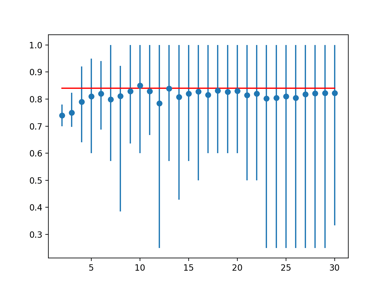
线图:交叉验证 k 值的平均准确率(带误差线,蓝色)与理想情况(红色)
这提供了一个模板,您可以使用它来对所选模型在数据集上相对于给定理想测试条件的 k 值的敏感性进行分析。
测试设备与目标的关联度
一旦选择了测试设备,另一个考虑因素是它在不同算法中与理想测试条件的匹配程度。
对于某些算法和某些配置,k 折交叉验证可能比其他算法和算法配置更接近理想测试条件。
我们可以明确地评估和报告这种关系。这可以通过计算一系列算法的 k 折交叉验证结果与同一算法在理想测试条件上的评估的匹配程度来实现。
可以计算两组分数之间的皮尔逊相关系数来衡量它们有多接近。也就是说,它们是否以相同的方式一起变化:当一种算法通过 k 折交叉验证看起来优于另一种算法时,这在理想测试条件上也成立吗?
我们期望看到分数之间存在很强的正相关,例如 0.5 或更高。低相关性表明需要更改 k 折交叉验证测试设备以更好地匹配理想测试条件。
首先,我们可以定义一个函数,该函数将创建一系列标准机器学习模型,以通过每个测试设备进行评估。
|
1 2 3 4 5 6 7 8 9 10 11 12 13 14 15 16 17 18 19 20 21 22 |
# 获取要评估的模型列表 定义 获取_模型(): models = list() models.append(LogisticRegression()) models.append(RidgeClassifier()) models.append(SGDClassifier()) models.append(PassiveAggressiveClassifier()) models.append(KNeighborsClassifier()) models.append(DecisionTreeClassifier()) models.append(ExtraTreeClassifier()) models.append(LinearSVC()) models.append(SVC()) models.append(GaussianNB()) models.append(AdaBoostClassifier()) models.append(BaggingClassifier()) models.append(RandomForestClassifier()) models.append(ExtraTreesClassifier()) models.append(GaussianProcessClassifier()) models.append(GradientBoostingClassifier()) models.append(LinearDiscriminantAnalysis()) models.append(QuadraticDiscriminantAnalysis()) 返回 models |
我们将 k=10 用于选择的测试设备。
然后我们可以枚举每个模型,并使用 10 折交叉验证和我们的理想测试条件(在本例中为 LOOCV)对其进行评估。
|
1 2 3 4 5 6 7 8 9 10 11 12 13 14 15 16 17 18 19 20 21 |
... # 定义测试条件 ideal_cv = LeaveOneOut() cv = KFold(n_splits=10, shuffle=True, random_state=1) # 获取要考虑的模型列表 模型 = 获取_模型() # 收集结果 ideal_results, cv_results = list(), list() # 评估每个模型 for model in models: # 使用每个测试条件评估模型 cv_mean = evaluate_model(cv, model) ideal_mean = evaluate_model(ideal_cv, model) # 检查无效结果 if isnan(cv_mean) or isnan(ideal_mean): continue # 存储结果 cv_results.append(cv_mean) ideal_results.append(ideal_mean) # 总结进度 print('>%s: ideal=%.3f, cv=%.3f' % (type(model).__name__, ideal_mean, cv_mean)) |
然后,我们可以计算 10 折交叉验证测试设备中的平均分类准确率与 LOOCV 测试设备之间的相关性。
|
1 2 3 4 |
... # 计算每个测试条件之间的相关性 corr, _ = pearsonr(cv_results, ideal_results) print('Correlation: %.3f' % corr) |
最后,我们可以创建两个结果集散点图,并绘制最佳拟合线,以直观地了解它们如何协同变化。
|
1 2 3 4 5 6 7 8 9 |
... # 结果散点图 pyplot.scatter(cv_results, ideal_results) # 绘制最佳拟合线 coeff, bias = polyfit(cv_results, ideal_results, 1) line = coeff * asarray(cv_results) + bias pyplot.plot(cv_results, line, color='r') # 显示绘图 pyplot.show() |
将所有这些联系在一起,完整的示例如下。
|
1 2 3 4 5 6 7 8 9 10 11 12 13 14 15 16 17 18 19 20 21 22 23 24 25 26 27 28 29 30 31 32 33 34 35 36 37 38 39 40 41 42 43 44 45 46 47 48 49 50 51 52 53 54 55 56 57 58 59 60 61 62 63 64 65 66 67 68 69 70 71 72 73 74 75 76 77 78 79 80 81 82 83 84 85 86 87 88 89 90 91 92 93 94 95 96 97 98 99 100 101 102 |
# 测试平台与理想测试条件之间的相关性 from numpy import mean from numpy import isnan from numpy import asarray from numpy import polyfit from scipy.stats import pearsonr from matplotlib import pyplot from sklearn.datasets import make_classification from sklearn.model_selection import KFold from sklearn.model_selection import LeaveOneOut from sklearn.model_selection import cross_val_score from sklearn.linear_model import LogisticRegression from sklearn.linear_model import RidgeClassifier from sklearn.linear_model import SGDClassifier from sklearn.linear_model import PassiveAggressiveClassifier from sklearn.neighbors import KNeighborsClassifier from sklearn.tree import DecisionTreeClassifier from sklearn.tree import ExtraTreeClassifier 从 sklearn.svm 导入 LinearSVC from sklearn.svm import SVC from sklearn.naive_bayes import GaussianNB from sklearn.ensemble import AdaBoostClassifier from sklearn.ensemble import BaggingClassifier from sklearn.ensemble import RandomForestClassifier from sklearn.ensemble import ExtraTreesClassifier from sklearn.gaussian_process import GaussianProcessClassifier from sklearn.ensemble import GradientBoostingClassifier from sklearn.discriminant_analysis import LinearDiscriminantAnalysis from sklearn.discriminant_analysis import QuadraticDiscriminantAnalysis # 创建数据集 def get_dataset(n_samples=100): X, y = make_classification(n_samples=n_samples, n_features=20, n_informative=15, n_redundant=5, random_state=1) 返回 X, y # 获取要评估的模型列表 定义 获取_模型(): models = list() models.append(LogisticRegression()) models.append(RidgeClassifier()) models.append(SGDClassifier()) models.append(PassiveAggressiveClassifier()) models.append(KNeighborsClassifier()) models.append(DecisionTreeClassifier()) models.append(ExtraTreeClassifier()) models.append(LinearSVC()) models.append(SVC()) models.append(GaussianNB()) models.append(AdaBoostClassifier()) models.append(BaggingClassifier()) models.append(RandomForestClassifier()) models.append(ExtraTreesClassifier()) models.append(GaussianProcessClassifier()) models.append(GradientBoostingClassifier()) models.append(LinearDiscriminantAnalysis()) models.append(QuadraticDiscriminantAnalysis()) 返回 模型 # 使用给定的测试条件评估模型 def evaluate_model(cv, model): # 获取数据集 X, y = get_dataset() # 评估模型 scores = cross_val_score(model, X, y, scoring='accuracy', cv=cv, n_jobs=-1) # 返回分数 return mean(scores) # 定义测试条件 ideal_cv = LeaveOneOut() cv = KFold(n_splits=10, shuffle=True, random_state=1) # 获取要考虑的模型列表 模型 = 获取_模型() # 收集结果 ideal_results, cv_results = list(), list() # 评估每个模型 for model in models: # 使用每个测试条件评估模型 cv_mean = evaluate_model(cv, model) ideal_mean = evaluate_model(ideal_cv, model) # 检查无效结果 if isnan(cv_mean) or isnan(ideal_mean): continue # 存储结果 cv_results.append(cv_mean) ideal_results.append(ideal_mean) # 总结进度 print('>%s: ideal=%.3f, cv=%.3f' % (type(model).__name__, ideal_mean, cv_mean)) # 计算每个测试条件之间的相关性 corr, _ = pearsonr(cv_results, ideal_results) print('Correlation: %.3f' % corr) # 结果散点图 pyplot.scatter(cv_results, ideal_results) # 绘制最佳拟合线 coeff, bias = polyfit(cv_results, ideal_results, 1) line = coeff * asarray(cv_results) + bias pyplot.plot(cv_results, line, color='r') # 标记图表 pyplot.title('10 折交叉验证 vs. 留一法交叉验证平均准确率') pyplot.xlabel('平均准确率 (10 折交叉验证)') pyplot.ylabel('平均准确率 (留一法交叉验证)') # 显示绘图 pyplot.show() |
运行示例会报告通过每种测试平台计算出的每种算法的平均分类准确率。
注意:由于算法或评估程序的随机性,或者数值精度的差异,您的结果可能不同。考虑运行几次示例并比较平均结果。
您可能会看到一些可以安全忽略的警告,例如
|
1 |
变量共线性 |
我们可以看到,对于某些算法,与留一法交叉验证相比,测试平台高估了准确率,而在其他情况下,它低估了准确率。这是可以预期的。
在运行结束时,我们可以看到报告了两个结果集之间的相关性。在这种情况下,我们可以看到报告了 0.746 的相关性,这是一个良好且强的正相关。结果表明,如通过 18 种流行机器学习算法计算所示,10 折交叉验证确实为该数据集上的留一法交叉验证测试平台提供了良好的近似。
|
1 2 3 4 5 6 7 8 9 10 11 12 13 14 15 16 17 18 19 |
>逻辑回归:理想=0.840, 交叉验证=0.850 >岭分类器:理想=0.830, 交叉验证=0.830 >SGDClassifier:理想=0.730, 交叉验证=0.790 >PassiveAggressiveClassifier:理想=0.780, 交叉验证=0.760 >KNeighborsClassifier:理想=0.760, 交叉验证=0.770 >DecisionTreeClassifier:理想=0.690, 交叉验证=0.630 >ExtraTreeClassifier:理想=0.710, 交叉验证=0.620 >LinearSVC:理想=0.850, 交叉验证=0.830 >SVC:理想=0.900, 交叉验证=0.880 >GaussianNB:理想=0.730, 交叉验证=0.720 >AdaBoostClassifier:理想=0.740, 交叉验证=0.740 >BaggingClassifier:理想=0.770, 交叉验证=0.740 >RandomForestClassifier:理想=0.810, 交叉验证=0.790 >ExtraTreesClassifier:理想=0.820, 交叉验证=0.820 >GaussianProcessClassifier:理想=0.790, 交叉验证=0.760 >GradientBoostingClassifier:理想=0.820, 交叉验证=0.820 >LinearDiscriminantAnalysis:理想=0.830, 交叉验证=0.830 >QuadraticDiscriminantAnalysis:理想=0.610, 交叉验证=0.760 相关性:0.746 |
最后,创建了散点图,比较了测试平台(x 轴)的平均准确率得分分布与留一法交叉验证(y 轴)的准确率得分。
绘制了一条红色的最佳拟合线,显示了强烈的线性相关性。
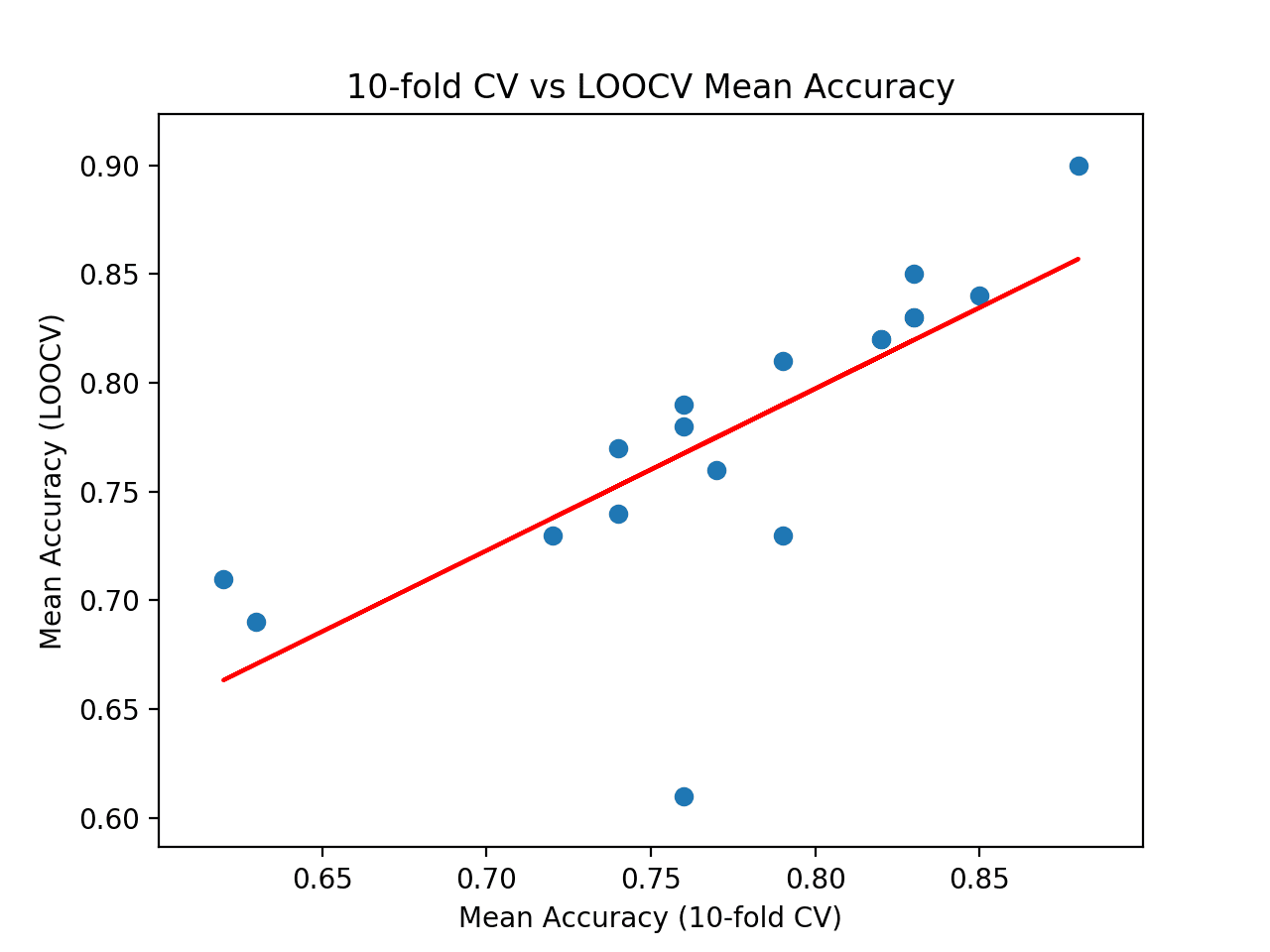
交叉验证与理想测试平均准确率散点图及最佳拟合线
这提供了一个平台,用于将您选择的测试平台与您自己数据集上的理想测试条件进行比较。
进一步阅读
如果您想深入了解,本节提供了更多关于该主题的资源。
教程
API
- sklearn.model_selection.KFold API.
- sklearn.model_selection.LeaveOneOut API.
- sklearn.model_selection.cross_val_score API.
文章
总结
在本教程中,您学习了如何配置和评估 k 折交叉验证的配置。
具体来说,你学到了:
- 如何使用 k 折交叉验证在数据集上评估机器学习算法。
- 如何对 k 折交叉验证的 k 值进行敏感性分析。
- 如何计算交叉验证测试设备与理想测试条件之间的相关性。
你有什么问题吗?
在下面的评论中提出你的问题,我会尽力回答。
发现 Python 中的快速机器学习!
在几分钟内开发您自己的模型
...只需几行 scikit-learn 代码
在我的新电子书中学习如何操作
精通 Python 机器学习
涵盖自学教程和端到端项目,例如
加载数据、可视化、建模、调优等等...
最终将机器学习带入
您自己的项目
跳过学术理论。只看结果。


再次感谢,这是一篇非常好的教程!
但是,在比较具有不同 n_splits 值的 kfold 结果时,我强烈建议使用除此处使用的误差以外的其他误差。
代码行是框中的第 52 行,该框以“# sensitivity analysis of k in k-fold cross-validation”开头。
事实上,正如您目前使用的 yerr=[mins, maxs] 一样,误差线的长度倾向于随着 n_splits 值的增加而增加,而我认为它实际上应该倾向于减小。我认为使用类似 yerr =[mean-std, mean+std] 的东西会更合适。如果您认为我错了,请告诉我。
不客气。
感谢您的建议。
有可能解释强化学习吗?
这是我在这里回答的一个常见问题
https://machinelearning.org.cn/faq/single-faq/do-you-have-tutorials-on-deep-reinforcement-learning
我如何在有两个文件夹的手语数据集上执行交叉验证,如果我想为训练执行九折,其余用于测试?
也许将所有数据加载到内存中,然后使用 sklearn 中的交叉验证类。
你好 Jason,
这是否可以用于像 lstm 这样的时间序列方法?
不,您必须使用前向验证
https://machinelearning.org.cn/backtest-machine-learning-models-time-series-forecasting/
尊敬的Jason博士,
在最后一个示例中,除了模型的平均值之外,
我还计算了理想和交叉验证分数的标准差。
结果和模型摘要,基于理想分数和交叉验证分数的标准差和平均值的最小/最大值
结论
可以看出,SVC 是模型的首选,其平均理想值为 0.9,交叉验证值为 0.80。相应的理想标准差为 0.3,交叉验证为 0.087。
根据交叉验证分数的最小变异性,KFold 的变异性最小,为 0.087,而留一法交叉验证的变异性为 0.3。
因此,对于该数据集,SVC 使用 KFold 交叉验证分数是最佳选择。
谢谢你,
悉尼的Anthony
很棒的实验!感谢分享您的发现。
Jason先生您好,
感谢您的大力支持。
我想问一下,如何使用 keras 中的 Imagedatagenerator 和 flow from directory 执行 k 折交叉验证?任何示例代码都能更清楚地理解。请指导。
此致
nkm
抱歉,我没有结合这两种方法的示例——我认为它们不兼容。
嗨 Jason,您是否为每种超参数的可能组合运行 k 的敏感性分析?例如
对于所有可能的超参数
运行 Loocv
运行 k 的敏感性分析
谢谢 🙂
不,使用 10。
本教程旨在帮助您理解为什么在大多数情况下我们选择 3、5 或 10。
您好,谢谢 🙂
我想知道,您是否对每个算法使用相同的“cv”对象?这是否意味着,在训练每个算法时(当您使用 cross_val_score() 时),训练/测试的拆分是每次都完全相同的?
也就是说,逻辑回归将与高斯朴素贝叶斯等进行相同的 10 折训练和测试,对吗?
谢谢你
好问题。
我想您说得对,为每个模型重新创建对象会更清晰。为了安全起见,我建议进行此更改。
嗨,Jason,
感谢您提供的精彩教程和直觉。我在一个具有大约 1500 个特征(少于 10k 条记录)的数据集上试用了您的代码,它非常慢……我的意思是,处理了几天。所以我想知道我是否应该做些不同的事情,或者……它不适用于这样的数据集。谢谢
这些建议将有所帮助
https://machinelearning.org.cn/faq/single-faq/how-do-i-speed-up-the-training-of-my-model
您好,当您在每次 k 迭代中打印每个 k 的准确率时,您正在运行 k 折。这意味着总共有 k*k 折,而不仅仅是 k 折,对吗?如果我的问题有意义的话。
正确,它是 k 个结果的平均值。
你好Jason,请告诉我,当我们使用k折交叉验证标准时,是否需要将模型拟合到完整的X和Y数据上,而不是将其拆分为训练集和测试集,对吗?其次,我在一些文章中看到人们在cross_val_score中使用xtrain和ytrain,而不是x和y,这有什么逻辑吗?
是的,k折交叉验证用于替代训练/测试拆分。
也许可以问问你正在阅读的其他教程的作者他们的原因。
如果我使用5折,我能从每一折中获得最大的测试准确率,然后将这5个最大准确率的平均值作为我的最终分数用于深度神经网络吗?
不,取平均值。取最大值是无效的。
你好,
感谢这篇精彩的文章和整个博客!
我仍然不确定我们是否应该使用LOOCV作为“地面真实”(即理想测试)来定义我们的最佳k。我特别困惑的是“结果表明,也许k=10本身有点乐观,而k=13可能是一个更准确的估计。”
1)当我查看k=7的图表时,很难得出结论。在我看来,所有平均分数都接近红色曲线,并且显示出很大的变异性。
2)由于我们没有显示LOOCV得分的最小值/最大值,所以我们不知道我们的模型(即ML方法+参数化)是否稳定(即使在这里可能不是这种情况)。
此致 Alexis
不客气。
同意,这只是一个地面真实的方法。
你好 Jason,
非常感谢“machinelearningmastery.com”上的精彩系列文章。
我正在使用python sci-kit learn进行信号处理实验。我有一个详细的问题,涉及到K折交叉验证和后续预测的多个步骤。我将在下面描述它们。
我有8640个信号数据样本,我将其分为训练集(70%)和验证集(30%)。这给了我6048个训练样本和2592个验证样本。我将验证样本进一步细分——2500个样本用于K折交叉验证,92个样本作为未见过/实时信号。我的最终目标是正确预测所有92个未见过/实时样本。
我将在下面提供一个代码片段。
estimator = KerasClassifier(build_fn=lambda: model, epochs=350, batch_size=32, verbose=1)
estimator.fit(X_train, Y_train) //这是6048个样本
kfold = KFold(n_splits=10, shuffle=True)
results = cross_val_score(estimator, X_test[0:2500,:], Y_test[0:2500], cv=kfold)
print(“Accuracy: %.2f%% (%.2f%%)” % (results.mean()*100, results.std()*100))
predictions = estimator.predict(X_test[2400:2492,:]) #这些是已经用于K折的测试样本
print(predictions)
predictions-2 = estimator.predict(X_test[2500:2592,:]) #这些是完全未见过的样本
print(predictions-2)
我的结果是
1.准确率(K折交叉验证)= 70%
2.准确率的标准差 = 29%
3.从2400到2492的所有样本都已正确预测
4.在2500到2592的样本中,只有12个样本被正确预测。
我想知道,是不是我理解错了什么。为什么只有少数未见过的样本被正确预测,即使所有用于K折的样本都已正确预测?
此致,
斯瓦蒂。
也许选择的测试框架不适合您的数据,您可以尝试其他配置?
也许您正在使用的模型或数据准备对您的数据不是最有效的,也许您可以探索其他替代方案?
好文!
另外,我对这一行有点困惑,
´´´scores = cross_val_score(model, X, y, scoring=’accuracy’, cv=cv, n_jobs=-1)
`我认为这模糊了k折交叉验证的功能和实际用法,并限制了代码的可定制性。
所以我做了一些代码修改,以展示一个执行相同任务的“分步手动方法”。
希望它能有所帮助。
这是我的建议
´´´
# 导入 ———————————————————————-
import numpy as np # Math, Stat and Linear Algebra python library
from sklearn.datasets import make_classification # Random generator for classification data
from sklearn.model_selection import KFold # k-Fold module
from sklearn.model_selection import cross_val_score # k-Fold Cross Validation fully automated module
from sklearn.linear_model import LogisticRegression # Model: Logistic Regression module
# 参数 ——————————————————————-
k = 10 # 折数 (k折交叉验证中的“k”值)
n_samples = 100 # 样本数
n_features = 20 # 数据特征数
# 定义数据集 —————————————————————
X, y = make_classification(n_samples=n_samples, n_features=n_features, n_informative=15, n_redundant=5, random_state=1)
# X的形状为(100, 20),y的形状为(100,)
# -> X包含浮点数值
# -> y仅包含0或1值
# -> 示例:X_i -> y_i := [1.123, … , 0.123123] -> 0或1
# 初始化逻辑回归模型和KFold ——————————————
model = LogisticRegression()
kfold = KFold(n_splits=k, random_state=1, shuffle=True)
# 学习和k折交叉验证:全自动化 ———————————————
# -> 所有操作都由sklearn模块“cross_val_score”完成
scores = cross_val_score(model, X, y, scoring=’accuracy’, cv=kfold, n_jobs=-1)
print(“全自动化方法: “)
print(” 准确率: μ = {0}, σ = {1}”.format( round(np.mean(scores), 3), round(np.std(scores),3) ))
# 学习和k折交叉验证:手动 ———————————————
# -> k折交叉验证过程的分步分解
scores = []
for train_index, test_index in kfold.split(X)
# 定义k折的测试和训练数据
X_train, X_test = X[train_index], X[test_index]
y_train, y_test = y[train_index], y[test_index]
# 在训练数据上训练逻辑回归模型
model.fit(X_train, y_train)
# 使用训练好的模型预测测试数据上的输出(y)
y_pred = model.predict(X_test)
# 计算模型在测试数据上的准确率
n_correct_values = sum([ p == t for p, t in zip(y_pred, y_test) ])
accuracy = n_correct_values / len(y_pred)
scores.append(accuracy)
scores = np.array(scores)
print(“手动方法: “)
print(” 准确率: μ = {0}, σ = {1}”.format( round(np.mean(scores), 3), round(np.std(scores),3) ))
´´´
PS:我不知道如何在此网站上发布python代码。非常抱歉。
我没有检查你的代码,但谢谢你的建议。
为什么(KFOLD)在执行时显示相同的结果?
import os
import time
import re
#import numpy as np
import pandas as pd
import matplotlib.pyplot as plt
from tqdm import tqdm
from sklearn.feature_extraction.text import CountVectorizer, TfidfVectorizer
from sklearn import preprocessing
from sklearn.model_selection import train_test_split, StratifiedKFold, KFold
from sklearn.naive_bayes import MultinomialNB
from sklearn.linear_model import SGDClassifier
from sklearn.linear_model import LogisticRegression
from sklearn.svm import LinearSVC
from sklearn.ensemble import RandomForestClassifier, GradientBoostingClassifier
from sklearn.metrics import classification_report
from sklearn.metrics import confusion_matrix
from sklearn.metrics import plot_confusion_matrix
from sklearn.metrics import precision_recall_fscore_support as score
df = pd.read_excel(‘/content/arabic (7).xlsx’)
df.head()
x = df[‘text’]
y = df[‘sen’]
from sklearn.feature_extraction.text import CountVectorizer
count_vect = CountVectorizer()
X_train_counts = count_vect.fit_transform(x)
X_train_counts.shape
from sklearn.feature_extraction.text import TfidfTransformer
tfidf_transformer = TfidfTransformer()
X_train_tfidf = tfidf_transformer.fit_transform(X_train_counts)
X_train_tfidf.shape
from sklearn.preprocessing import LabelEncoder
df=df.dropna()
le=LabelEncoder()
df[‘sen’]=le.fit_transform(df[‘sen’])
df.head()
y=df[‘sen’]
model =LinearSVC()
fold_no=10
K=10
skf = StratifiedKFold(n_splits=10)
def training(train, test, fold_no)
x_train = X_train_tfidf
y_train=y
x_test = X_train_tfidf
y_test =y
model.fit(x_train, y_train)
score = model.score(x_test,y_test)
print(‘For Fold {} the accuracy is {}’.format(str(fold_no),score))
fold_no = 1
acc_score = []
for train_index,test_index in skf.split(x, y)
train = df.iloc[train_index,:]
test = df.iloc[test_index,:]
training(train, test, fold_no)
fold_no += 1
———-OUTPUT———-
For Fold 1 the accuracy is 0.9251433994965543
For Fold 2 the accuracy is 0.9251433994965543
For Fold 3 the accuracy is 0.9251433994965543
For Fold 4 the accuracy is 0.9251433994965543
For Fold 5 the accuracy is 0.9251433994965543
For Fold 6 the accuracy is 0.9251433994965543
For Fold 7 the accuracy is 0.9251433994965543
For Fold 8 the accuracy is 0.9251433994965543
For Fold 9 the accuracy is 0.9251433994965543
For Fold 10 the accuracy is 0.9251433994965543
也许您的问题很简单,或者您的代码有错误。
感谢Jason博士的精彩博客。您能否帮助实现两个输入和一个输出的K折交叉验证?我的实现如下所示
num_folds = 5
kfold = StratifiedKFold(n_splits=num_folds, shuffle=True)
for IDs_Train, IDs_Test in kfold.split(X_CXR,y_CXR)
X1_train_cv, X2_train_cv = X_CT[IDs_Train], X_CXR[IDs_Train]
y1_train_cv = y_CT[IDs_Train]
X1_test_cv, X2_test_cv = X_CT[IDs_Test], X_CXR[IDs_Test]
y1_test_cv = y_CT[IDs_Test]
此外,我在model.fit中使用了validation_split = 0.2
问题:我的验证准确率在初始的许多迭代中保持为0,并且增长非常缓慢,导致过拟合,尽管它在单折实现中没有过拟合(取得了良好的测试准确率)。
恳请指导。
此致
为什么不先将两个输入合并到一个数组或DataFrame中,然后再应用StratifiedKFold?
感谢您的快速回复。它帮助很大。非常感谢。
你好Adrian博士,
我还有另一个疑问。当我进行5折交叉验证时,我是否需要为每一折重新初始化模型/网络的权重?我注意到,随着它从第一折进展到最后一折,过拟合会增加,这可能是由于权重溢出到下一折。
如果答案是肯定的,我该如何做到?
谢谢并致以问候
是的。分别处理这5折,不要共享任何初始化等。
只需在每一折循环的开始重新创建模型,并进行拟合和验证。
感谢您的快速回复。我正在尝试您的方法。此外,我只是在for循环的每一折结束时删除模型变量(del model)。这是正确的方法吗??
再次感谢。
正确。但您可能不需要删除模型,而只需在每个循环开始时创建一个新模型就足够了。
非常感谢您快速而准确的解决方案。感谢您的支持,您是一位“真正的向导”。
所以,每当我们使用交叉验证时,我们会提供整个数据集,它会为我们进行训练、测试和验证吗?对吗?
下一个问题是,当我们使用交叉验证时,如何使用模型来预测新样本?有predict函数吗?
任何回复都将受到赞赏。
祝好,
你好Fereshteh……以下内容可能会有所帮助
https://machinelearning.org.cn/training-validation-test-split-and-cross-validation-done-right/
谢谢
sa
skf = StratifiedKFold(n_splits=3, shuffle=True, random_state=1)
lst_accu_stratified = []
labels = {‘AD’:0, ‘SZP’:1, }
ad_sz[‘class_number’] = ad_sz[‘target’]
ad_sz.class_number = [labels[item] for item in ad_sz.class_number]
ad_sz[‘class_number’] = ad_sz[‘class_number’].astype(np.float32)
# 将目标转换为数值型
# 定义输入和输出数据集
input = ad_sz.iloc[:, 0]
print(‘\n输入值是:’)
print(input.head())
output = ad_sz.loc[:, ‘class_number’]
print(‘\n输出值是:’)
print(output.head())
input = torch.from_numpy(np.vstack(input).astype(np.float32)) # 创建张量
print(‘\n输入格式: ‘, input.shape, input.dtype)
output = torch.tensor(output.values) # 创建张量
print(‘输出格式: ‘, output.shape, output.dtype)
data_ = TensorDataset(input, output)
model = LogisticRegression(solver=’lbfgs’,max_iter=1000)
skf = StratifiedKFold(n_splits=4, shuffle=True, random_state=1)
lst_accu_stratified = []
for train_index, test_index in skf.split(input, output)
X_train_fold, X_test_fold = input[train_index], input[test_index]
y_train_fold, y_test_fold = output[train_index], output[test_index]
model.fit(X_train_fold, y_train_fold)
lst_accu_stratified.append(model.score(X_test_fold, y_test_fold))
print(‘最大准确率’,max(lst_accu_stratified))
print(‘最小准确率:’,min(lst_accu_stratified))
print(‘总体准确率:’,mean(lst_accu_stratified))
from sklearn.metrics import plot_confusion_matrix
plot_confusion_matrix(model, X_train_fold,y_train_fold)
对于以上内容,我正在尝试遵循分层k折并打印准确率、灵敏度和特异性
我卡在如何打印准确率、灵敏度和特异性上了,有什么想法吗?
你好Koundinya……以下内容可能会让你感兴趣
https://www.analyticsvidhya.com/blog/2021/06/classification-problem-relation-between-sensitivity-specificity-and-accuracy/
有没有办法让验证集的大小始终为20%,而不考虑折数?
嗨,Jason,
我如何将您的代码应用于CNN模型而不是随机森林?我定义了我的模型架构如下:
def get_model()
xinput=kl.Input((200,9,1))
#添加高斯噪声以减少过拟合()
xNoise=kl.GaussianNoise(.005)(xinput)
#仅在时间序列方向上进行卷积(类似于过滤)
x1=kl.Conv2D(NUMBER_FILTERS,(SIZE_FILTERS,1),kernel_regularizer=keras.regularizers.L1(l1=REG))(xNoise)
#合并信息
x1=kl.Conv2D(NUMBER_FILTERS,(SIZE_FILTERS,1),kernel_regularizer=keras.regularizers.L1(l1=REG),activation=’gelu’)(x1)
xFeatures=kl.Conv2D(DIMENSION_SUBSPACE1,(1,1),kernel_regularizer=keras.regularizers.L1(l1=REG),activation=’gelu’)(x1)
#全局池化(网络对平移不变)
xP=tf.reduce_max(xFeatures,axis=1)
#低维空间分类器
x2=kl.Flatten()(xP)
x2=kl.Dense(DIMENSION_SUBSPACE2,activation=’gelu’)(x2)
xout=kl.Dense(1,activation=’sigmoid’)(x2)
return keras.Model(xinput,xout)
#model_Interpretation=keras.Model(xinput,xFeatures)
这是摘要
Model: “model”
_________________________________________________________________
层(类型) 输出形状 参数 #
=================================================================
input_1 (InputLayer) [(None, 200, 9, 1)] 0
gaussian_noise (GaussianNo (None, 200, 9, 1) 0
ise)
conv2d (Conv2D) (None, 186, 9, 32) 512
conv2d_1 (Conv2D) (None, 172, 9, 32) 15392
conv2d_2 (Conv2D) (None, 172, 9, 3) 99
tf.math.reduce_max (TFOpLa (None, 9, 3) 0
mbda)
flatten (Flatten) (None, 27) 0
dense (Dense) (None, 3) 84
dense_1 (Dense) (None, 1) 4
=================================================================
总参数:16091(62.86 KB)
可训练参数:16091(62.86 KB)
不可训练参数:0(0.00 Byte)
这是编译和训练模型的代码行
model.compile(optimizer=keras.optimizers.Adam(learning_rate=.001),loss=’binary_crossentropy’,metrics=’accuracy’)
CB=[keras.callbacks.ReduceLROnPlateau(monitor=’loss’,patience=10),keras.callbacks.EarlyStopping(monitor=’loss’,patience=30,restore_best_weights=True)]
model.fit(X,Y,batch_size=4,epochs=600,callbacks=CB)
我一直在尝试实现您的代码,但我不知道如何操作。感谢您的任何帮助,并为我的蹩脚英语道歉。
谢谢 🙂
你好Carlos……请提供您遇到的任何错误消息的文本。这将使我们能够更好地为您提供建议。