指数平滑是一种用于单变量数据的时间序列预测方法,可以扩展以支持具有系统趋势或季节性分量的数据。
通常的做法是使用优化过程来查找模型超参数,这些超参数能够使指数平滑模型在给定时间序列数据集上表现最佳。这种做法仅适用于模型用于描述水平、趋势和季节性的指数结构的系数。
还可以自动优化指数平滑模型的其他超参数,例如是否对趋势和季节性分量进行建模,以及如果进行建模,是使用加法还是乘法方法对其进行建模。
在本教程中,您将学习如何开发一个框架,用于对单变量时间序列预测的所有指数平滑模型超参数进行网格搜索。
完成本教程后,您将了解:
- 如何从头开始使用向前验证开发一个网格搜索 ETS 模型的框架。
- 如何对每日女性出生时间序列数据进行 ETS 模型超参数网格搜索。
- 如何对洗发水销量、汽车销量和温度的每月时间序列数据进行 ETS 模型超参数网格搜索。
通过我的新书《时间序列预测深度学习》启动您的项目,其中包括分步教程和所有示例的 Python 源代码文件。
让我们开始吧。
- 2018 年 10 月更新:更新了 ETS 模型的拟合以使用 NumPy 数组,修复了乘法趋势/季节性问题(感谢 Amit Amola)。
- 2019 年 4 月更新:更新了数据集链接。

如何在 Python 中对三重指数平滑时间序列预测进行网格搜索
图片由 john mcsporran 提供,保留部分权利。
教程概述
本教程分为六个部分;它们是:
- 时间序列预测中的指数平滑
- 开发网格搜索框架
- 案例研究 1:无趋势或季节性
- 案例研究 2:趋势
- 案例研究 3:季节性
- 案例研究 4:趋势和季节性
时间序列预测中的指数平滑
指数平滑是一种用于单变量数据的时间序列预测方法。
像 Box-Jenkins ARIMA 系列方法这样的时间序列方法开发了一个模型,其中预测是近期过去观测或滞后的加权线性和。
指数平滑预测方法类似,预测是过去观测的加权和,但模型明确地对过去观测使用指数递减的权重。
具体来说,过去观测值以几何递减的比率进行加权。
使用指数平滑方法产生的预测是过去观测值的加权平均值,权重随着观测值的变旧而呈指数衰减。换句话说,观测值越新,相关的权重就越高。
— 第 171 页,《预测:原理与实践》,2013 年。
指数平滑方法可以被认为是时间序列预测中流行的 Box-Jenkins ARIMA 类方法的同类和替代方案。
总的来说,这些方法有时被称为 ETS 模型,指的是对误差、趋势和季节性的显式建模。
指数平滑分为三种类型:
- 单一指数平滑,或 SES,用于没有趋势或季节性的单变量数据。
- 双重指数平滑,用于支持趋势的单变量数据。
- 三重指数平滑,或 Holt-Winters 指数平滑,支持趋势和季节性。
三重指数平滑模型通过配置趋势的性质(加法、乘法或无)和季节性的性质(加法、乘法或无),以及任何趋势的阻尼,涵盖了单一和双重指数平滑。
时间序列深度学习需要帮助吗?
立即参加我为期7天的免费电子邮件速成课程(附示例代码)。
点击注册,同时获得该课程的免费PDF电子书版本。
开发网格搜索框架
在本节中,我们将开发一个框架,用于对给定单变量时间序列预测问题的指数平滑模型超参数进行网格搜索。
我们将使用 statsmodels 库提供的 Holt-Winters 指数平滑实现。
该模型具有控制序列、趋势和季节性执行的指数性质的超参数,具体如下:
- smoothing_level (alpha):水平的平滑系数。
- smoothing_slope (beta):趋势的平滑系数。
- smoothing_seasonal (gamma):季节性分量的平滑系数。
- damping_slope (phi):阻尼趋势的系数。
所有这四个超参数都可以在定义模型时指定。如果未指定,库将自动调整模型并找到这些超参数的最佳值(例如,optimized=True)。
模型不会自动调整的其他超参数,您可能希望指定:
- trend:趋势分量的类型,可以是“add”(加法)或“mul”(乘法)。通过将其设置为 None 可以禁用趋势建模。
- damped:趋势分量是否应该被阻尼,可以是 True 或 False。
- seasonal:季节性分量的类型,可以是“add”(加法)或“mul”(乘法)。通过将其设置为 None 可以禁用季节性分量建模。
- seasonal_periods:一个季节性周期中的时间步数,例如,每年季节性结构中的 12 个月。
- use_boxcox:是否对序列执行幂变换(True/False),或指定变换的 lambda 值。
如果您对您的问题有足够的了解以指定这些参数中的一个或多个,那么您应该指定它们。如果不是,您可以尝试对这些参数进行网格搜索。
我们可以首先定义一个函数,该函数将用给定的配置拟合模型并进行一步预测。
下面的 exp_smoothing_forecast() 实现了此行为。
该函数接受一个连续的先前观测值数组或列表,以及一个用于配置模型的配置参数列表。
配置参数按顺序是:趋势类型、阻尼类型、季节性类型、季节周期、是否使用 Box-Cox 变换,以及拟合模型时是否去除偏差。
|
1 2 3 4 5 6 7 8 9 10 11 |
# 一步 Holt-Winters 指数平滑预测 def exp_smoothing_forecast(history, config): t,d,s,p,b,r = config # 定义模型 history = array(history) model = ExponentialSmoothing(history, trend=t, damped=d, seasonal=s, seasonal_periods=p) # 拟合模型 model_fit = model.fit(optimized=True, use_boxcox=b, remove_bias=r) # 进行一步预测 yhat = model_fit.predict(len(history), len(history)) return yhat[0] |
接下来,我们需要构建一些函数,用于通过向前验证重复拟合和评估模型,包括将数据集拆分为训练集和测试集以及评估一步预测。
我们可以使用给定指定拆分大小(例如,在测试集中使用数据的时间步数)的切片来拆分列表或 NumPy 数组数据。
下面的 train_test_split() 函数为给定数据集和测试集中要使用的指定时间步数实现了此功能。
|
1 2 3 |
# 将单变量数据集拆分为训练/测试集 def train_test_split(data, n_test): return data[:-n_test], data[-n_test:] |
在对测试数据集中的每个步骤进行预测后,需要将它们与测试集进行比较以计算误差分数。
时间序列预测有许多流行的误差分数。在这种情况下,我们将使用均方根误差 (RMSE),但您可以将其更改为您首选的度量,例如 MAPE、MAE 等。
下面的 *measure_rmse()* 函数将根据实际值(测试集)和预测值列表计算 RMSE。
|
1 2 3 |
# 均方根误差或 RMSE def measure_rmse(actual, predicted): return sqrt(mean_squared_error(actual, predicted)) |
我们现在可以实现向前验证方案。这是一种评估时间序列预测模型的标准方法,它尊重观测的时间顺序。
首先,使用 train_test_split() 函数将给定的单变量时间序列数据集拆分为训练集和测试集。然后枚举测试集中的观测数量。对于每个观测,我们基于所有历史数据拟合一个模型并进行一步预测。然后将该时间步的真实观测添加到历史数据中,并重复此过程。调用 exp_smoothing_forecast() 函数以拟合模型并进行预测。最后,通过调用 measure_rmse() 函数,将所有一步预测与实际测试集进行比较,计算误差分数。
下面的 walk_forward_validation() 函数实现了这一点,它接受一个单变量时间序列、测试集中要使用的时间步数以及一个模型配置数组。
|
1 2 3 4 5 6 7 8 9 10 11 12 13 14 15 16 17 18 |
# 单变量数据的滚动预测验证 def walk_forward_validation(data, n_test, cfg): predictions = list() # 拆分数据集 train, test = train_test_split(data, n_test) # 用训练数据集初始化历史数据 history = [x for x in train] # 遍历测试集中的每个时间步 for i in range(len(test)): # 拟合模型并对历史数据进行预测 yhat = exp_smoothing_forecast(history, cfg) # 将预测结果存储在预测列表中 predictions.append(yhat) # 将实际观测值添加到历史数据中以进行下一次循环 history.append(test[i]) # 估计预测误差 error = measure_rmse(test, predictions) return error |
如果您有兴趣进行多步预测,您可以更改 exp_smoothing_forecast() 函数中对 predict() 的调用,并更改 measure_rmse() 函数中误差的计算。
我们可以使用不同的模型配置列表重复调用 *walk_forward_validation()*。
一个可能的问题是,某些模型配置组合可能不会被模型调用,并会引发异常,例如,指定数据中季节性结构的一些但不全部方面。
此外,某些模型在某些数据上也可能引发警告,例如来自 statsmodels 库调用的线性代数库。
我们可以通过将所有对 walk_forward_validation() 的调用包装在 try-except 块中,并添加一个忽略警告的块,来捕获异常并忽略网格搜索期间的警告。我们还可以添加调试支持来禁用这些保护,以防我们想查看真实情况。最后,如果发生错误,我们可以返回 None 结果;否则,我们可以打印有关每个评估模型技能的一些信息。这在评估大量模型时很有用。
下面的 score_model() 函数实现了这一点,并返回一个 (key, result) 元组,其中 key 是测试模型配置的字符串版本。
|
1 2 3 4 5 6 7 8 9 10 11 12 13 14 15 16 17 18 19 20 21 |
# 评估模型,失败时返回 None def score_model(data, n_test, cfg, debug=False): result = None # 将配置转换为键 key = str(cfg) # 如果在调试,则显示所有警告并在异常时失败 if debug: result = walk_forward_validation(data, n_test, cfg) else: # 模型验证过程中的一次失败表明配置不稳定 try: # 网格搜索时从不显示警告,太嘈杂 with catch_warnings(): filterwarnings("ignore") result = walk_forward_validation(data, n_test, cfg) except: error = None # 检查是否有有趣的结果 if result is not None: print(' > Model[%s] %.3f' % (key, result)) return (key, result) |
接下来,我们需要一个循环来测试不同的模型配置列表。
这是驱动网格搜索过程的主要函数,它将为每个模型配置调用 *score_model()* 函数。
我们可以通过并行评估模型配置来显著加快网格搜索过程。一种方法是使用 Joblib 库。
我们可以定义一个 Parallel 对象,并设置要使用的核心数,将其设置为您的硬件中检测到的 CPU 核心数。
|
1 |
executor = Parallel(n_jobs=cpu_count(), backend='multiprocessing') |
然后我们可以创建一个并行执行任务的列表,对于我们拥有的每个模型配置,这将是对 score_model() 函数的一次调用。
|
1 |
tasks = (delayed(score_model)(data, n_test, cfg) for cfg in cfg_list) |
最后,我们可以使用 Parallel 对象并行执行任务列表。
|
1 |
scores = executor(tasks) |
就是这样。
我们还可以提供一个非并行版本的模型配置评估,以防我们想要调试某些东西。
|
1 |
scores = [score_model(data, n_test, cfg) for cfg in cfg_list] |
评估配置列表的结果将是一个元组列表,每个元组包含一个总结特定模型配置的名称以及以 RMSE 或 None(如果发生错误)表示的模型误差。
我们可以过滤掉所有分数为 None 的项。
|
1 |
scores = [r for r in scores if r[1] != None] |
然后我们可以按升序(最佳在前)对列表中所有元组进行排序,然后返回此分数列表以供审查。
下面的 grid_search() 函数实现了此行为,给定一个单变量时间序列数据集、一个模型配置列表(列表的列表)以及测试集中要使用的时间步数。可选的 parallel 参数允许打开或关闭所有核心上的模型评估,默认为打开。
|
1 2 3 4 5 6 7 8 9 10 11 12 13 14 15 |
# 网格搜索配置 def grid_search(data, cfg_list, n_test, parallel=True): scores = None if parallel: # 并行执行配置 executor = Parallel(n_jobs=cpu_count(), backend='multiprocessing') tasks = (delayed(score_model)(data, n_test, cfg) for cfg in cfg_list) scores = executor(tasks) else: scores = [score_model(data, n_test, cfg) for cfg in cfg_list] # 移除空结果 scores = [r for r in scores if r[1] != None] # 按误差升序排序配置 scores.sort(key=lambda tup: tup[1]) return scores |
我们快完成了。
剩下的唯一一件事是定义要用于数据集的模型配置列表。
我们可以泛化地定义它。我们可能想指定的唯一参数是序列中季节性分量的周期性(如果存在)。默认情况下,我们将假设没有季节性分量。
下面的 exp_smoothing_configs() 函数将创建一个要评估的模型配置列表。
可以指定一个可选的季节周期列表,您甚至可以更改函数以指定您可能了解的时间序列的其他元素。
理论上,有 72 种可能的模型配置需要评估,但实际上,许多配置无效,将导致我们捕获并忽略的错误。
|
1 2 3 4 5 6 7 8 9 10 11 12 13 14 15 16 17 18 19 20 |
# 创建一组要尝试的指数平滑配置 def exp_smoothing_configs(seasonal=[None]): models = list() # 定义配置列表 t_params = ['add', 'mul', None] d_params = [True, False] s_params = ['add', 'mul', None] p_params = seasonal b_params = [True, False] r_params = [True, False] # 创建配置实例 for t in t_params: for d in d_params: for s in s_params: for p in p_params: for b in b_params: forr in r_params: cfg = [t,d,s,p,b,r] models.append(cfg) 返回 models |
我们现在有了一个通过一步向前验证网格搜索三重指数平滑模型超参数的框架。
它是通用的,适用于作为列表或 NumPy 数组提供的任何内存中单变量时间序列。
我们可以通过在一个构造的 10 步数据集上测试它来确保所有部分协同工作。
完整的示例如下所示。
|
1 2 3 4 5 6 7 8 9 10 11 12 13 14 15 16 17 18 19 20 21 22 23 24 25 26 27 28 29 30 31 32 33 34 35 36 37 38 39 40 41 42 43 44 45 46 47 48 49 50 51 52 53 54 55 56 57 58 59 60 61 62 63 64 65 66 67 68 69 70 71 72 73 74 75 76 77 78 79 80 81 82 83 84 85 86 87 88 89 90 91 92 93 94 95 96 97 98 99 100 101 102 103 104 105 106 107 108 109 110 111 112 113 114 115 116 117 118 119 120 121 122 123 |
# 网格搜索 Holt-Winter 指数平滑 from math import sqrt from multiprocessing import cpu_count from joblib import Parallel from joblib import delayed from warnings import catch_warnings from warnings import filterwarnings from statsmodels.tsa.holtwinters import ExponentialSmoothing from sklearn.metrics import mean_squared_error from numpy import array # 一步 Holt Winter 指数平滑预测 def exp_smoothing_forecast(history, config): t,d,s,p,b,r = config # 定义模型 history = array(history) model = ExponentialSmoothing(history, trend=t, damped=d, seasonal=s, seasonal_periods=p) # 拟合模型 model_fit = model.fit(optimized=True, use_boxcox=b, remove_bias=r) # 进行一步预测 yhat = model_fit.predict(len(history), len(history)) return yhat[0] # 均方根误差或 RMSE def measure_rmse(actual, predicted): return sqrt(mean_squared_error(actual, predicted)) # 将单变量数据集拆分为训练/测试集 def train_test_split(data, n_test): return data[:-n_test], data[-n_test:] # 单变量数据的滚动预测验证 def walk_forward_validation(data, n_test, cfg): predictions = list() # 拆分数据集 train, test = train_test_split(data, n_test) # 用训练数据集初始化历史数据 history = [x for x in train] # 遍历测试集中的每个时间步 for i in range(len(test)): # 拟合模型并对历史数据进行预测 yhat = exp_smoothing_forecast(history, cfg) # 将预测结果存储在预测列表中 predictions.append(yhat) # 将实际观测值添加到历史数据中以进行下一次循环 history.append(test[i]) # 估计预测误差 error = measure_rmse(test, predictions) return error # 评估模型,失败时返回 None def score_model(data, n_test, cfg, debug=False): result = None # 将配置转换为键 key = str(cfg) # 如果在调试,则显示所有警告并在异常时失败 if debug: result = walk_forward_validation(data, n_test, cfg) else: # 模型验证过程中的一次失败表明配置不稳定 try: # 网格搜索时从不显示警告,太嘈杂 with catch_warnings(): filterwarnings("ignore") result = walk_forward_validation(data, n_test, cfg) except: error = None # 检查是否有有趣的结果 if result is not None: print(' > Model[%s] %.3f' % (key, result)) return (key, result) # 网格搜索配置 def grid_search(data, cfg_list, n_test, parallel=True): scores = None if parallel: # 并行执行配置 executor = Parallel(n_jobs=cpu_count(), backend='multiprocessing') tasks = (delayed(score_model)(data, n_test, cfg) for cfg in cfg_list) scores = executor(tasks) else: scores = [score_model(data, n_test, cfg) for cfg in cfg_list] # 移除空结果 scores = [r for r in scores if r[1] != None] # 按误差升序排序配置 scores.sort(key=lambda tup: tup[1]) 返回 分数 # 创建一组要尝试的指数平滑配置 def exp_smoothing_configs(seasonal=[None]): models = list() # 定义配置列表 t_params = ['add', 'mul', None] d_params = [True, False] s_params = ['add', 'mul', None] p_params = seasonal b_params = [True, False] r_params = [True, False] # 创建配置实例 for t in t_params: for d in d_params: for s in s_params: for p in p_params: for b in b_params: forr in r_params: cfg = [t,d,s,p,b,r] models.append(cfg) return models if __name__ == '__main__': # 定义数据集 data = [10.0, 20.0, 30.0, 40.0, 50.0, 60.0, 70.0, 80.0, 90.0, 100.0] print(data) # 数据分割 n_test = 4 # 模型配置 cfg_list = exp_smoothing_configs() # 网格搜索 scores = grid_search(data, cfg_list, n_test) print('完成') # 列出前 3 个配置 for cfg, error in scores[:3]: print(cfg, error) |
运行示例首先打印人工生成的时间序列数据集。
接下来,模型配置及其误差将随着评估而报告。
最后,报告前三个配置的配置和误差。
|
1 2 3 4 5 6 7 8 9 10 11 |
[10.0, 20.0, 30.0, 40.0, 50.0, 60.0, 70.0, 80.0, 90.0, 100.0] > 模型[[None, False, None, None, True, True]] 1.380 > 模型[[None, False, None, None, True, False]] 10.000 > 模型[[None, False, None, None, False, True]] 2.563 > 模型[[None, False, None, None, False, False]] 10.000 完成 [None, False, None, None, True, True] 1.379824445857423 [None, False, None, None, False, True] 2.5628662672606612 [None, False, None, None, False, False] 10.0 |
我们不报告模型本身优化的模型参数。假设您可以通过指定更宽泛的超参数并允许库找到相同的内部参数来再次获得相同的结果。
您可以通过使用相同的配置重新拟合独立模型并打印模型拟合上的“params”属性的内容来访问这些内部参数;例如
|
1 |
print(model_fit.params) |
现在我们有了网格搜索ETS模型超参数的强大框架,让我们在一些标准单变量时间序列数据集上进行测试。
数据集是出于演示目的而选择的;我并不是说ETS模型是每个数据集的最佳方法,在某些情况下,SARIMA或其他方法可能更合适。
案例研究 1:无趋势或季节性
“每日女性出生人数”数据集汇总了 1959 年美国加利福尼亚州每日女性出生总数。
该数据集没有明显的趋势或季节性成分。
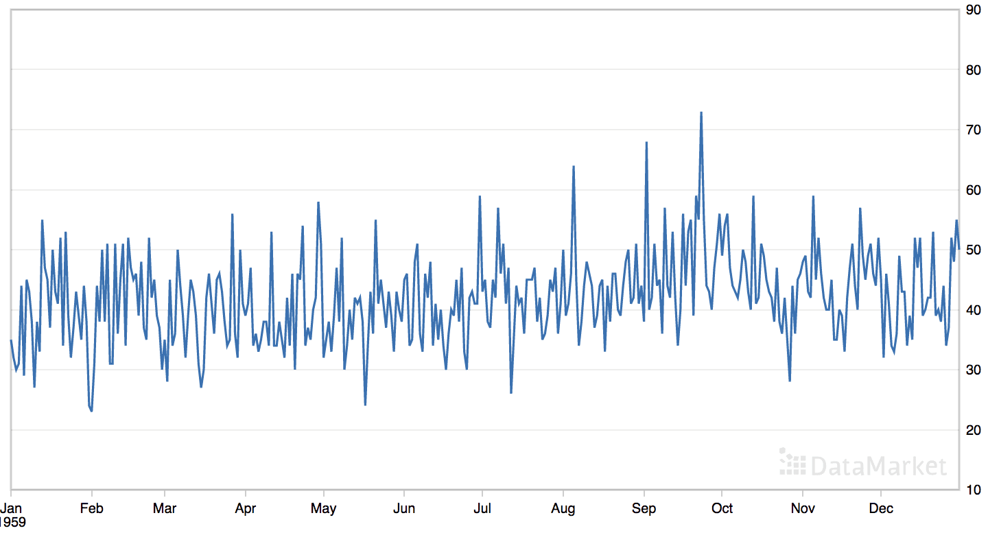
每日女性出生人数数据集的线图
直接从这里下载数据集
将文件保存为“_daily-total-female-births.csv_”在当前工作目录中。
我们可以使用 *read_csv()* 函数将此数据集加载为 Pandas 序列。
|
1 |
series = read_csv('daily-total-female-births.csv', header=0, index_col=0) |
数据集有一年,即 365 个观测值。我们将使用前 200 个进行训练,其余 165 个作为测试集。
下面列出了对每日女性单变量时间序列预测问题进行网格搜索的完整示例。
|
1 2 3 4 5 6 7 8 9 10 11 12 13 14 15 16 17 18 19 20 21 22 23 24 25 26 27 28 29 30 31 32 33 34 35 36 37 38 39 40 41 42 43 44 45 46 47 48 49 50 51 52 53 54 55 56 57 58 59 60 61 62 63 64 65 66 67 68 69 70 71 72 73 74 75 76 77 78 79 80 81 82 83 84 85 86 87 88 89 90 91 92 93 94 95 96 97 98 99 100 101 102 103 104 105 106 107 108 109 110 111 112 113 114 115 116 117 118 119 120 121 122 123 124 |
# 网格搜索每日女性出生数的ETS模型 from math import sqrt from multiprocessing import cpu_count from joblib import Parallel from joblib import delayed from warnings import catch_warnings from warnings import filterwarnings from statsmodels.tsa.holtwinters import ExponentialSmoothing from sklearn.metrics import mean_squared_error from pandas import read_csv from numpy import array # 一步 Holt Winter 指数平滑预测 def exp_smoothing_forecast(history, config): t,d,s,p,b,r = config # 定义模型 history = array(history) model = ExponentialSmoothing(history, trend=t, damped=d, seasonal=s, seasonal_periods=p) # 拟合模型 model_fit = model.fit(optimized=True, use_boxcox=b, remove_bias=r) # 进行一步预测 yhat = model_fit.predict(len(history), len(history)) return yhat[0] # 均方根误差或 RMSE def measure_rmse(actual, predicted): return sqrt(mean_squared_error(actual, predicted)) # 将单变量数据集拆分为训练/测试集 def train_test_split(data, n_test): return data[:-n_test], data[-n_test:] # 单变量数据的滚动预测验证 def walk_forward_validation(data, n_test, cfg): predictions = list() # 拆分数据集 train, test = train_test_split(data, n_test) # 用训练数据集初始化历史数据 history = [x for x in train] # 遍历测试集中的每个时间步 for i in range(len(test)): # 拟合模型并对历史数据进行预测 yhat = exp_smoothing_forecast(history, cfg) # 将预测结果存储在预测列表中 predictions.append(yhat) # 将实际观测值添加到历史数据中以进行下一次循环 history.append(test[i]) # 估计预测误差 error = measure_rmse(test, predictions) return error # 评估模型,失败时返回 None def score_model(data, n_test, cfg, debug=False): result = None # 将配置转换为键 key = str(cfg) # 如果在调试,则显示所有警告并在异常时失败 if debug: result = walk_forward_validation(data, n_test, cfg) else: # 模型验证过程中的一次失败表明配置不稳定 try: # 网格搜索时从不显示警告,太嘈杂 with catch_warnings(): filterwarnings("ignore") result = walk_forward_validation(data, n_test, cfg) except: error = None # 检查是否有有趣的结果 if result is not None: print(' > Model[%s] %.3f' % (key, result)) return (key, result) # 网格搜索配置 def grid_search(data, cfg_list, n_test, parallel=True): scores = None if parallel: # 并行执行配置 executor = Parallel(n_jobs=cpu_count(), backend='multiprocessing') tasks = (delayed(score_model)(data, n_test, cfg) for cfg in cfg_list) scores = executor(tasks) else: scores = [score_model(data, n_test, cfg) for cfg in cfg_list] # 移除空结果 scores = [r for r in scores if r[1] != None] # 按误差升序排序配置 scores.sort(key=lambda tup: tup[1]) 返回 分数 # 创建一组要尝试的指数平滑配置 def exp_smoothing_configs(seasonal=[None]): models = list() # 定义配置列表 t_params = ['add', 'mul', None] d_params = [True, False] s_params = ['add', 'mul', None] p_params = seasonal b_params = [True, False] r_params = [True, False] # 创建配置实例 for t in t_params: for d in d_params: for s in s_params: for p in p_params: for b in b_params: forr in r_params: cfg = [t,d,s,p,b,r] models.append(cfg) return models if __name__ == '__main__': # 加载数据集 series = read_csv('daily-total-female-births.csv', header=0, index_col=0) data = series.values # 数据分割 n_test = 165 # 模型配置 cfg_list = exp_smoothing_configs() # 网格搜索 scores = grid_search(data[:,0], cfg_list, n_test) print('完成') # 列出前 3 个配置 for cfg, error in scores[:3]: print(cfg, error) |
运行此示例可能需要几分钟,因为在现代硬件上拟合每个ETS模型可能需要大约一分钟。
模型配置和RMSE将在模型评估时打印出来。运行结束时将报告前三个模型配置及其误差。
注意:由于算法或评估过程的随机性,或数值精度的差异,您的结果可能会有所不同。考虑运行示例几次并比较平均结果。
我们可以看到,最佳结果是RMSE约为6.96次出生,配置如下
- 趋势:乘法
- 阻尼:False
- 季节性:None
- 季节周期:None
- Box-Cox 变换:True
- 去除偏差:True
令人惊讶的是,假设乘法趋势的模型表现优于不假设的模型。
除非我们抛弃假设并网格搜索模型,否则我们不会知道这种情况。
|
1 2 3 4 5 6 7 8 9 10 11 12 13 14 15 16 17 18 19 20 21 22 23 |
> 模型[['add', False, None, None, True, True]] 7.081 > 模型[['add', False, None, None, True, False]] 7.113 > 模型[['add', False, None, None, False, True]] 7.112 > 模型[['add', False, None, None, False, False]] 7.115 > 模型[['add', True, None, None, True, True]] 7.118 > 模型[['add', True, None, None, True, False]] 7.170 > 模型[['add', True, None, None, False, True]] 7.113 > 模型[['add', True, None, None, False, False]] 7.126 > 模型[['mul', True, None, None, True, True]] 7.118 > 模型[['mul', True, None, None, True, False]] 7.170 > 模型[['mul', True, None, None, False, True]] 7.113 > 模型[['mul', True, None, None, False, False]] 7.126 > 模型[['mul', False, None, None, True, True]] 6.961 > 模型[['mul', False, None, None, True, False]] 6.985 > 模型[[None, False, None, None, True, True]] 7.169 > 模型[[None, False, None, None, True, False]] 7.212 > 模型[[None, False, None, None, False, True]] 7.117 > 模型[[None, False, None, None, False, False]] 7.126 完成 ['mul', False, None, None, True, True] 6.960703917145126 ['mul', False, None, None, True, False] 6.984513598720297 ['add', False, None, None, True, True] 7.081359856193836 |
案例研究 2:趋势
“洗发水”数据集汇总了三年期间洗发水的月销售额。
该数据集包含一个明显的趋势,但没有明显的季节性成分。
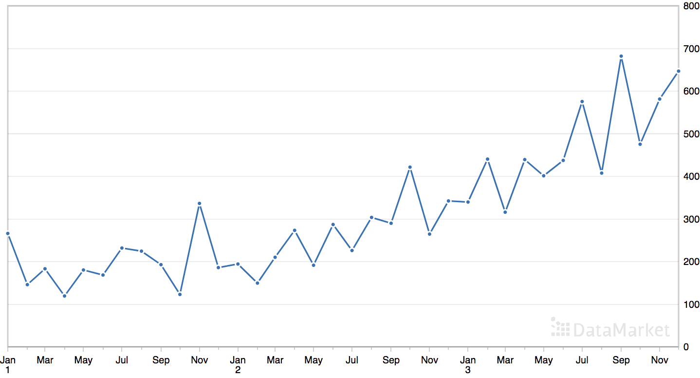
月度洗发水销售数据集的线图
直接从这里下载数据集
将文件保存为当前工作目录中的“shampoo.csv”。
我们可以使用 *read_csv()* 函数将此数据集加载为 Pandas 序列。
|
1 2 3 4 5 6 |
# 解析日期 def custom_parser(x): return datetime.strptime('195'+x, '%Y-%m') # 加载数据集 series = read_csv('shampoo.csv', header=0, index_col=0, date_parser=custom_parser) |
数据集有三年,即 36 个观测值。我们将使用前 24 个进行训练,其余 12 个作为测试集。
下面列出了对洗发水销售单变量时间序列预测问题进行网格搜索的完整示例。
|
1 2 3 4 5 6 7 8 9 10 11 12 13 14 15 16 17 18 19 20 21 22 23 24 25 26 27 28 29 30 31 32 33 34 35 36 37 38 39 40 41 42 43 44 45 46 47 48 49 50 51 52 53 54 55 56 57 58 59 60 61 62 63 64 65 66 67 68 69 70 71 72 73 74 75 76 77 78 79 80 81 82 83 84 85 86 87 88 89 90 91 92 93 94 95 96 97 98 99 100 101 102 103 104 105 106 107 108 109 110 111 112 113 114 115 116 117 118 119 120 121 122 123 124 |
# 网格搜索月度洗发水销量的 ETS 模型 from math import sqrt from multiprocessing import cpu_count from joblib import Parallel from joblib import delayed from warnings import catch_warnings from warnings import filterwarnings from statsmodels.tsa.holtwinters import ExponentialSmoothing from sklearn.metrics import mean_squared_error from pandas import read_csv from numpy import array # 一步 Holt Winter 指数平滑预测 def exp_smoothing_forecast(history, config): t,d,s,p,b,r = config # 定义模型 history = array(history) model = ExponentialSmoothing(history, trend=t, damped=d, seasonal=s, seasonal_periods=p) # 拟合模型 model_fit = model.fit(optimized=True, use_boxcox=b, remove_bias=r) # 进行一步预测 yhat = model_fit.predict(len(history), len(history)) return yhat[0] # 均方根误差或 RMSE def measure_rmse(actual, predicted): return sqrt(mean_squared_error(actual, predicted)) # 将单变量数据集拆分为训练/测试集 def train_test_split(data, n_test): return data[:-n_test], data[-n_test:] # 单变量数据的滚动预测验证 def walk_forward_validation(data, n_test, cfg): predictions = list() # 拆分数据集 train, test = train_test_split(data, n_test) # 用训练数据集初始化历史数据 history = [x for x in train] # 遍历测试集中的每个时间步 for i in range(len(test)): # 拟合模型并对历史数据进行预测 yhat = exp_smoothing_forecast(history, cfg) # 将预测结果存储在预测列表中 predictions.append(yhat) # 将实际观测值添加到历史数据中以进行下一次循环 history.append(test[i]) # 估计预测误差 error = measure_rmse(test, predictions) return error # 评估模型,失败时返回 None def score_model(data, n_test, cfg, debug=False): result = None # 将配置转换为键 key = str(cfg) # 如果在调试,则显示所有警告并在异常时失败 if debug: result = walk_forward_validation(data, n_test, cfg) else: # 模型验证过程中的一次失败表明配置不稳定 try: # 网格搜索时从不显示警告,太嘈杂 with catch_warnings(): filterwarnings("ignore") result = walk_forward_validation(data, n_test, cfg) except: error = None # 检查是否有有趣的结果 if result is not None: print(' > Model[%s] %.3f' % (key, result)) return (key, result) # 网格搜索配置 def grid_search(data, cfg_list, n_test, parallel=True): scores = None if parallel: # 并行执行配置 executor = Parallel(n_jobs=cpu_count(), backend='multiprocessing') tasks = (delayed(score_model)(data, n_test, cfg) for cfg in cfg_list) scores = executor(tasks) else: scores = [score_model(data, n_test, cfg) for cfg in cfg_list] # 移除空结果 scores = [r for r in scores if r[1] != None] # 按误差升序排序配置 scores.sort(key=lambda tup: tup[1]) 返回 分数 # 创建一组要尝试的指数平滑配置 def exp_smoothing_configs(seasonal=[None]): models = list() # 定义配置列表 t_params = ['add', 'mul', None] d_params = [True, False] s_params = ['add', 'mul', None] p_params = seasonal b_params = [True, False] r_params = [True, False] # 创建配置实例 for t in t_params: for d in d_params: for s in s_params: for p in p_params: for b in b_params: forr in r_params: cfg = [t,d,s,p,b,r] models.append(cfg) return models if __name__ == '__main__': # 加载数据集 series = read_csv('shampoo.csv', header=0, index_col=0) data = series.values # 数据分割 n_test = 12 # 模型配置 cfg_list = exp_smoothing_configs() # 网格搜索 scores = grid_search(data[:,0], cfg_list, n_test) print('完成') # 列出前 3 个配置 for cfg, error in scores[:3]: print(cfg, error) |
由于观测值数量少,运行示例很快。
模型配置和RMSE将在模型评估时打印出来。运行结束时将报告前三个模型配置及其误差。
注意:由于算法或评估过程的随机性,或数值精度的差异,您的结果可能会有所不同。考虑运行示例几次并比较平均结果。
我们可以看到,最佳结果是RMSE约为83.74销量,配置如下
- 趋势:乘法
- 阻尼:False
- 季节性:None
- 季节周期:None
- Box-Cox 变换:False
- 去除偏差:False
|
1 2 3 4 5 6 7 8 9 10 11 12 13 14 15 |
> 模型[['add', False, None, None, False, True]] 106.431 > 模型[['add', False, None, None, False, False]] 104.874 > 模型[['add', True, None, None, False, False]] 103.069 > 模型[['add', True, None, None, False, True]] 97.918 > 模型[['mul', True, None, None, False, True]] 95.337 > 模型[['mul', True, None, None, False, False]] 102.152 > 模型[['mul', False, None, None, False, True]] 86.406 > 模型[['mul', False, None, None, False, False]] 83.747 > 模型[[None, False, None, None, False, True]] 99.416 > 模型[[None, False, None, None, False, False]] 108.031 完成 ['mul', False, None, None, False, False] 83.74666940175238 ['mul', False, None, None, False, True] 86.40648953786152 ['mul', True, None, None, False, True] 95.33737598817238 |
案例研究 3:季节性
“月平均气温”数据集总结了 1920 年至 1939 年间英国诺丁汉城堡的月平均气温(华氏度)。
该数据集具有明显的季节性成分,但没有明显的趋势。
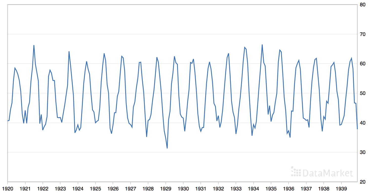
月平均气温数据集的线图
直接从这里下载数据集
将文件保存为当前工作目录中的“monthly-mean-temp.csv”。
我们可以使用 *read_csv()* 函数将此数据集加载为 Pandas 序列。
|
1 |
series = read_csv('monthly-mean-temp.csv', header=0, index_col=0) |
数据集有20年,即240个观测值。
我们将数据集裁剪为最近五年的数据(60个观测值),以加快模型评估过程,并使用最近一年(即12个观测值)作为测试集。
|
1 2 |
# 将数据集裁剪为 5 年 data = data[-(5*12):] |
季节分量的周期大约是一年,即12个观测值。
在准备模型配置时,我们将在调用`exp_smoothing_configs()`函数时使用此值作为季节周期。
|
1 2 |
# 模型配置 cfg_list = exp_smoothing_configs(seasonal=[0, 12]) |
下面列出了对月平均气温时间序列预测问题进行网格搜索的完整示例。
|
1 2 3 4 5 6 7 8 9 10 11 12 13 14 15 16 17 18 19 20 21 22 23 24 25 26 27 28 29 30 31 32 33 34 35 36 37 38 39 40 41 42 43 44 45 46 47 48 49 50 51 52 53 54 55 56 57 58 59 60 61 62 63 64 65 66 67 68 69 70 71 72 73 74 75 76 77 78 79 80 81 82 83 84 85 86 87 88 89 90 91 92 93 94 95 96 97 98 99 100 101 102 103 104 105 106 107 108 109 110 111 112 113 114 115 116 117 118 119 120 121 122 123 124 125 126 |
# 网格搜索月平均温度数据集的ETS超参数 from math import sqrt from multiprocessing import cpu_count from joblib import Parallel from joblib import delayed from warnings import catch_warnings from warnings import filterwarnings from statsmodels.tsa.holtwinters import ExponentialSmoothing from sklearn.metrics import mean_squared_error from pandas import read_csv from numpy import array # 一步 Holt Winter 指数平滑预测 def exp_smoothing_forecast(history, config): t,d,s,p,b,r = config # 定义模型 history = array(history) model = ExponentialSmoothing(history, trend=t, damped=d, seasonal=s, seasonal_periods=p) # 拟合模型 model_fit = model.fit(optimized=True, use_boxcox=b, remove_bias=r) # 进行一步预测 yhat = model_fit.predict(len(history), len(history)) return yhat[0] # 均方根误差或 RMSE def measure_rmse(actual, predicted): return sqrt(mean_squared_error(actual, predicted)) # 将单变量数据集拆分为训练/测试集 def train_test_split(data, n_test): return data[:-n_test], data[-n_test:] # 单变量数据的滚动预测验证 def walk_forward_validation(data, n_test, cfg): predictions = list() # 拆分数据集 train, test = train_test_split(data, n_test) # 用训练数据集初始化历史数据 history = [x for x in train] # 遍历测试集中的每个时间步 for i in range(len(test)): # 拟合模型并对历史数据进行预测 yhat = exp_smoothing_forecast(history, cfg) # 将预测结果存储在预测列表中 predictions.append(yhat) # 将实际观测值添加到历史数据中以进行下一次循环 history.append(test[i]) # 估计预测误差 error = measure_rmse(test, predictions) return error # 评估模型,失败时返回 None def score_model(data, n_test, cfg, debug=False): result = None # 将配置转换为键 key = str(cfg) # 如果在调试,则显示所有警告并在异常时失败 if debug: result = walk_forward_validation(data, n_test, cfg) else: # 模型验证过程中的一次失败表明配置不稳定 try: # 网格搜索时从不显示警告,太嘈杂 with catch_warnings(): filterwarnings("ignore") result = walk_forward_validation(data, n_test, cfg) except: error = None # 检查是否有有趣的结果 if result is not None: print(' > Model[%s] %.3f' % (key, result)) return (key, result) # 网格搜索配置 def grid_search(data, cfg_list, n_test, parallel=True): scores = None if parallel: # 并行执行配置 executor = Parallel(n_jobs=cpu_count(), backend='multiprocessing') tasks = (delayed(score_model)(data, n_test, cfg) for cfg in cfg_list) scores = executor(tasks) else: scores = [score_model(data, n_test, cfg) for cfg in cfg_list] # 移除空结果 scores = [r for r in scores if r[1] != None] # 按误差升序排序配置 scores.sort(key=lambda tup: tup[1]) 返回 分数 # 创建一组要尝试的指数平滑配置 def exp_smoothing_configs(seasonal=[None]): models = list() # 定义配置列表 t_params = ['add', 'mul', None] d_params = [True, False] s_params = ['add', 'mul', None] p_params = seasonal b_params = [True, False] r_params = [True, False] # 创建配置实例 for t in t_params: for d in d_params: for s in s_params: for p in p_params: for b in b_params: forr in r_params: cfg = [t,d,s,p,b,r] models.append(cfg) return models if __name__ == '__main__': # 加载数据集 series = read_csv('monthly-mean-temp.csv', header=0, index_col=0) data = series.values # 将数据集裁剪为5年 data = data[-(5*12):] # 数据分割 n_test = 12 # 模型配置 cfg_list = exp_smoothing_configs(seasonal=[0,12]) # 网格搜索 scores = grid_search(data[:,0], cfg_list, n_test) print('完成') # 列出前 3 个配置 for cfg, error in scores[:3]: print(cfg, error) |
鉴于数据量大,运行示例相对较慢。
模型配置和RMSE将在模型评估时打印出来。运行结束时将报告前三个模型配置及其误差。
注意:由于算法或评估过程的随机性,或数值精度的差异,您的结果可能会有所不同。考虑运行示例几次并比较平均结果。
我们可以看到,最佳结果是RMSE约为1.50度,配置如下
- 趋势:无
- 阻尼:False
- 季节性:加法
- 季节周期: 12
- Box-Cox 变换:False
- 去除偏差:False
|
1 2 3 4 5 6 7 8 9 10 11 12 13 14 15 16 17 18 19 20 21 22 23 24 25 26 27 28 29 30 31 32 33 34 35 36 37 38 39 40 41 42 43 44 45 46 47 48 49 50 51 52 53 54 55 56 57 58 59 60 61 62 63 64 65 66 67 68 69 70 71 72 73 74 75 76 77 |
> 模型[['add', True, 'mul', 12, True, False]] 1.659 > 模型[['add', True, 'mul', 12, True, True]] 1.663 > 模型[['add', True, 'mul', 12, False, True]] 1.603 > 模型[['add', True, 'mul', 12, False, False]] 1.609 > 模型[['mul', False, None, 0, True, True]] 4.920 > 模型[['mul', False, None, 0, True, False]] 4.881 > 模型[['mul', False, None, 0, False, True]] 4.838 > 模型[['mul', False, None, 0, False, False]] 4.813 > 模型[['add', True, 'add', 12, False, True]] 1.568 > 模型[['mul', False, None, 12, True, True]] 4.920 > 模型[['add', True, 'add', 12, False, False]] 1.555 > 模型[['add', True, 'add', 12, True, False]] 1.638 > 模型[['add', True, 'add', 12, True, True]] 1.646 > 模型[['mul', False, None, 12, True, False]] 4.881 > 模型[['mul', False, None, 12, False, True]] 4.838 > 模型[['mul', False, None, 12, False, False]] 4.813 > 模型[['add', True, None, 0, True, True]] 4.654 > 模型[[None, False, 'add', 12, True, True]] 1.508 > 模型[['add', True, None, 0, True, False]] 4.597 > 模型[['add', True, None, 0, False, True]] 4.800 > 模型[[None, False, 'add', 12, True, False]] 1.507 > 模型[['add', True, None, 0, False, False]] 4.760 > 模型[[None, False, 'add', 12, False, True]] 1.502 > 模型[['add', True, None, 12, True, True]] 4.654 > 模型[[None, False, 'add', 12, False, False]] 1.502 > 模型[['add', True, None, 12, True, False]] 4.597 > 模型[[None, False, 'mul', 12, True, True]] 1.507 > 模型[['add', True, None, 12, False, True]] 4.800 > 模型[[None, False, 'mul', 12, True, False]] 1.507 > 模型[['add', True, None, 12, False, False]] 4.760 > 模型[[None, False, 'mul', 12, False, True]] 1.502 > 模型[['add', False, 'add', 12, True, True]] 1.859 > 模型[[None, False, 'mul', 12, False, False]] 1.502 > 模型[[None, False, None, 0, True, True]] 5.188 > 模型[[None, False, None, 0, True, False]] 5.143 > 模型[[None, False, None, 0, False, True]] 5.187 > 模型[[None, False, None, 0, False, False]] 5.143 > 模型[[None, False, None, 12, True, True]] 5.188 > 模型[[None, False, None, 12, True, False]] 5.143 > 模型[[None, False, None, 12, False, True]] 5.187 > 模型[[None, False, None, 12, False, False]] 5.143 > 模型[['add', False, 'add', 12, True, False]] 1.825 > 模型[['add', False, 'add', 12, False, True]] 1.706 > 模型[['add', False, 'add', 12, False, False]] 1.710 > 模型[['add', False, 'mul', 12, True, True]] 1.882 > 模型[['add', False, 'mul', 12, True, False]] 1.739 > 模型[['add', False, 'mul', 12, False, True]] 1.580 > 模型[['add', False, 'mul', 12, False, False]] 1.581 > 模型[['add', False, None, 0, True, True]] 4.980 > 模型[['add', False, None, 0, True, False]] 4.900 > 模型[['add', False, None, 0, False, True]] 5.203 > 模型[['add', False, None, 0, False, False]] 5.151 > 模型[['add', False, None, 12, True, True]] 4.980 > 模型[['add', False, None, 12, True, False]] 4.900 > 模型[['add', False, None, 12, False, True]] 5.203 > 模型[['add', False, None, 12, False, False]] 5.151 > 模型[['mul', True, 'add', 12, True, True]] 19.353 > 模型[['mul', True, 'add', 12, True, False]] 9.807 > 模型[['mul', True, 'add', 12, False, True]] 11.696 > 模型[['mul', True, 'add', 12, False, False]] 2.847 > 模型[['mul', True, None, 0, True, True]] 4.607 > 模型[['mul', True, None, 0, True, False]] 4.570 > 模型[['mul', True, None, 0, False, True]] 4.630 > 模型[['mul', True, None, 0, False, False]] 4.596 > 模型[['mul', True, None, 12, True, True]] 4.607 > 模型[['mul', True, None, 12, True, False]] 4.570 > 模型[['mul', True, None, 12, False, True]] 4.630 > 模型[['mul', True, None, 12, False, False]] 4.593 > 模型[['mul', False, 'add', 12, True, True]] 4.230 > 模型[['mul', False, 'add', 12, True, False]] 4.157 > 模型[['mul', False, 'add', 12, False, True]] 1.538 > 模型[['mul', False, 'add', 12, False, False]] 1.520 完成 [None, False, 'add', 12, False, False] 1.5015527325330889 [None, False, 'add', 12, False, True] 1.5015531225114707 [None, False, 'mul', 12, False, False] 1.501561363221282 |
案例研究 4:趋势和季节性
“月度汽车销量”数据集总结了 1960 年至 1968 年间加拿大魁北克的月度汽车销量。
该数据集具有明显的趋势和季节性成分。
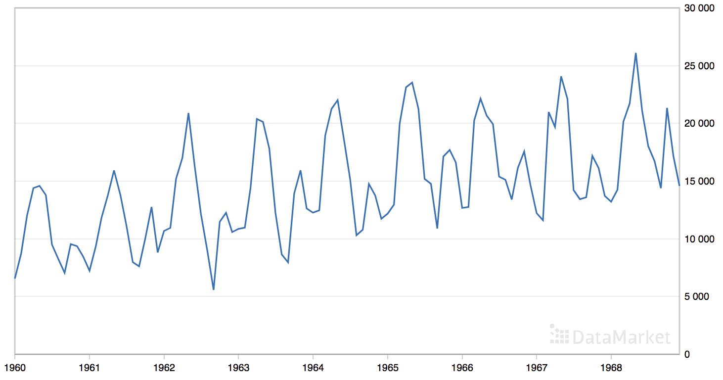
月度汽车销量数据集的线图
直接从这里下载数据集
将文件保存为当前工作目录中的“monthly-car-sales.csv”。
我们可以使用 *read_csv()* 函数将此数据集加载为 Pandas 序列。
|
1 |
series = read_csv('monthly-car-sales.csv', header=0, index_col=0) |
数据集有九年,即108个观测值。我们将使用最近一年,即12个观测值,作为测试集。
季节分量的周期可以是六个月或十二个月。在准备模型配置时,我们将在调用`exp_smoothing_configs()`函数时将两者都作为季节周期进行尝试。
|
1 2 |
# 模型配置 cfg_list = exp_smoothing_configs(seasonal=[0,6,12]) |
下面列出了对月度汽车销量时间序列预测问题进行网格搜索的完整示例。
|
1 2 3 4 5 6 7 8 9 10 11 12 13 14 15 16 17 18 19 20 21 22 23 24 25 26 27 28 29 30 31 32 33 34 35 36 37 38 39 40 41 42 43 44 45 46 47 48 49 50 51 52 53 54 55 56 57 58 59 60 61 62 63 64 65 66 67 68 69 70 71 72 73 74 75 76 77 78 79 80 81 82 83 84 85 86 87 88 89 90 91 92 93 94 95 96 97 98 99 100 101 102 103 104 105 106 107 108 109 110 111 112 113 114 115 116 117 118 119 120 121 122 123 124 |
# 网格搜索月度汽车销量的ETS模型 from math import sqrt from multiprocessing import cpu_count from joblib import Parallel from joblib import delayed from warnings import catch_warnings from warnings import filterwarnings from statsmodels.tsa.holtwinters import ExponentialSmoothing from sklearn.metrics import mean_squared_error from pandas import read_csv from numpy import array # 一步 Holt Winter 指数平滑预测 def exp_smoothing_forecast(history, config): t,d,s,p,b,r = config # 定义模型 history = array(history) model = ExponentialSmoothing(history, trend=t, damped=d, seasonal=s, seasonal_periods=p) # 拟合模型 model_fit = model.fit(optimized=True, use_boxcox=b, remove_bias=r) # 进行一步预测 yhat = model_fit.predict(len(history), len(history)) return yhat[0] # 均方根误差或 RMSE def measure_rmse(actual, predicted): return sqrt(mean_squared_error(actual, predicted)) # 将单变量数据集拆分为训练/测试集 def train_test_split(data, n_test): return data[:-n_test], data[-n_test:] # 单变量数据的滚动预测验证 def walk_forward_validation(data, n_test, cfg): predictions = list() # 拆分数据集 train, test = train_test_split(data, n_test) # 用训练数据集初始化历史数据 history = [x for x in train] # 遍历测试集中的每个时间步 for i in range(len(test)): # 拟合模型并对历史数据进行预测 yhat = exp_smoothing_forecast(history, cfg) # 将预测结果存储在预测列表中 predictions.append(yhat) # 将实际观测值添加到历史数据中以进行下一次循环 history.append(test[i]) # 估计预测误差 error = measure_rmse(test, predictions) return error # 评估模型,失败时返回 None def score_model(data, n_test, cfg, debug=False): result = None # 将配置转换为键 key = str(cfg) # 如果在调试,则显示所有警告并在异常时失败 if debug: result = walk_forward_validation(data, n_test, cfg) else: # 模型验证过程中的一次失败表明配置不稳定 try: # 网格搜索时从不显示警告,太嘈杂 with catch_warnings(): filterwarnings("ignore") result = walk_forward_validation(data, n_test, cfg) except: error = None # 检查是否有有趣的结果 if result is not None: print(' > Model[%s] %.3f' % (key, result)) return (key, result) # 网格搜索配置 def grid_search(data, cfg_list, n_test, parallel=True): scores = None if parallel: # 并行执行配置 executor = Parallel(n_jobs=cpu_count(), backend='multiprocessing') tasks = (delayed(score_model)(data, n_test, cfg) for cfg in cfg_list) scores = executor(tasks) else: scores = [score_model(data, n_test, cfg) for cfg in cfg_list] # 移除空结果 scores = [r for r in scores if r[1] != None] # 按误差升序排序配置 scores.sort(key=lambda tup: tup[1]) 返回 分数 # 创建一组要尝试的指数平滑配置 def exp_smoothing_configs(seasonal=[None]): models = list() # 定义配置列表 t_params = ['add', 'mul', None] d_params = [True, False] s_params = ['add', 'mul', None] p_params = seasonal b_params = [True, False] r_params = [True, False] # 创建配置实例 for t in t_params: for d in d_params: for s in s_params: for p in p_params: for b in b_params: forr in r_params: cfg = [t,d,s,p,b,r] models.append(cfg) return models if __name__ == '__main__': # 加载数据集 series = read_csv('monthly-car-sales.csv', header=0, index_col=0) data = series.values # 数据分割 n_test = 12 # 模型配置 cfg_list = exp_smoothing_configs(seasonal=[0,6,12]) # 网格搜索 scores = grid_search(data[:,0], cfg_list, n_test) print('完成') # 列出前 3 个配置 for cfg, error in scores[:3]: print(cfg, error) |
鉴于数据量大,运行示例速度较慢。
模型配置和RMSE将在模型评估时打印出来。运行结束时将报告前三个模型配置及其误差。
注意:由于算法或评估过程的随机性,或数值精度的差异,您的结果可能会有所不同。考虑运行示例几次并比较平均结果。
我们可以看到,最佳结果是RMSE约为1,672销量,配置如下
- 趋势:加法
- 阻尼:False
- 季节性:加法
- 季节周期: 12
- Box-Cox 变换:False
- 去除偏差:True
这有点令人惊讶,我本以为六个月的季节性模型会是首选方法。
|
1 2 3 4 5 6 7 8 9 10 11 12 13 14 15 16 17 18 19 20 21 22 23 24 25 26 27 28 29 30 31 32 33 34 35 36 37 38 39 40 41 42 43 44 45 46 47 48 49 50 51 52 53 54 55 56 57 58 59 60 61 62 63 64 65 66 67 68 69 70 71 72 73 74 75 76 77 78 79 80 81 82 83 84 85 86 87 88 89 90 91 92 93 94 95 96 97 98 99 100 101 102 103 104 105 106 107 108 109 110 111 112 113 114 115 116 117 118 119 120 121 122 123 124 125 126 127 128 129 130 131 132 133 134 |
> 模型[['add', True, 'add', 6, False, True]] 3240.433 > 模型[['add', True, 'add', 6, False, False]] 3226.384 > 模型[['add', True, 'add', 6, True, False]] 2836.535 > 模型[['add', True, 'add', 6, True, True]] 2784.852 > 模型[['add', True, 'add', 12, False, False]] 1696.173 > 模型[['add', True, 'add', 12, False, True]] 1721.746 > 模型[[None, False, 'add', 6, True, True]] 3204.874 > 模型[['add', True, 'add', 12, True, False]] 2064.937 > 模型[['add', True, 'add', 12, True, True]] 2098.844 > 模型[[None, False, 'add', 6, True, False]] 3190.972 > 模型[[None, False, 'add', 6, False, True]] 3147.623 > 模型[[None, False, 'add', 6, False, False]] 3126.527 > 模型[[None, False, 'add', 12, True, True]] 1834.910 > 模型[[None, False, 'add', 12, True, False]] 1872.081 > 模型[[None, False, 'add', 12, False, True]] 1736.264 > 模型[[None, False, 'add', 12, False, False]] 1807.325 > 模型[[None, False, 'mul', 6, True, True]] 2993.566 > 模型[[None, False, 'mul', 6, True, False]] 2979.123 > 模型[[None, False, 'mul', 6, False, True]] 3025.876 > 模型[[None, False, 'mul', 6, False, False]] 3009.999 > 模型[['add', True, 'mul', 6, True, True]] 2956.728 > 模型[[None, False, 'mul', 12, True, True]] 1972.547 > 模型[[None, False, 'mul', 12, True, False]] 1989.234 > 模型[[None, False, 'mul', 12, False, True]] 1925.010 > 模型[[None, False, 'mul', 12, False, False]] 1941.217 > 模型[[None, False, None, 0, True, True]] 3801.741 > 模型[[None, False, None, 0, True, False]] 3783.966 > 模型[[None, False, None, 0, False, True]] 3801.560 > 模型[[None, False, None, 0, False, False]] 3783.966 > 模型[[None, False, None, 6, True, True]] 3801.741 > 模型[[None, False, None, 6, True, False]] 3783.966 > 模型[[None, False, None, 6, False, True]] 3801.560 > 模型[[None, False, None, 6, False, False]] 3783.966 > 模型[[None, False, None, 12, True, True]] 3801.741 > 模型[[None, False, None, 12, True, False]] 3783.966 > 模型[[None, False, None, 12, False, True]] 3801.560 > 模型[[None, False, None, 12, False, False]] 3783.966 > 模型[['add', True, 'mul', 6, True, False]] 2932.827 > 模型[['mul', True, 'mul', 12, True, True]] 1953.405 > 模型[['add', True, 'mul', 6, False, True]] 2997.259 > 模型[['mul', True, 'mul', 12, True, False]] 1960.242 > 模型[['add', True, 'mul', 6, False, False]] 2979.248 > 模型[['mul', True, 'mul', 12, False, True]] 1907.792 > 模型[['add', True, 'mul', 12, True, True]] 1972.550 > 模型[['add', True, 'mul', 12, True, False]] 1989.236 > 模型[['mul', True, None, 0, True, True]] 3951.024 > 模型[['mul', True, None, 0, True, False]] 3930.394 > 模型[['mul', True, None, 0, False, True]] 3947.281 > 模型[['mul', True, None, 0, False, False]] 3926.082 > 模型[['mul', True, None, 6, True, True]] 3951.026 > 模型[['mul', True, None, 6, True, False]] 3930.389 > 模型[['mul', True, None, 6, False, True]] 3946.654 > 模型[['mul', True, None, 6, False, False]] 3926.026 > 模型[['mul', True, None, 12, True, True]] 3951.027 > 模型[['mul', True, None, 12, True, False]] 3930.368 > 模型[['mul', True, None, 12, False, True]] 3942.037 > 模型[['mul', True, None, 12, False, False]] 3920.756 > 模型[['add', True, 'mul', 12, False, True]] 1750.480 > 模型[['mul', False, 'add', 6, True, False]] 5043.557 > 模型[['mul', False, 'add', 6, False, True]] 7425.711 > 模型[['mul', False, 'add', 6, False, False]] 7448.455 > 模型[['mul', False, 'add', 12, True, True]] 2160.794 > 模型[['mul', False, 'add', 12, True, False]] 2346.478 > 模型[['mul', False, 'add', 12, False, True]] 16303.868 > 模型[['mul', False, 'add', 12, False, False]] 10268.636 > 模型[['mul', False, 'mul', 12, True, True]] 3012.036 > 模型[['mul', False, 'mul', 12, True, False]] 3005.824 > 模型[['add', True, 'mul', 12, False, False]] 1774.636 > 模型[['mul', False, 'mul', 12, False, True]] 14676.476 > 模型[['add', True, None, 0, True, True]] 3935.674 > 模型[['mul', False, 'mul', 12, False, False]] 13988.754 > 模型[['mul', False, None, 0, True, True]] 3804.906 > 模型[['mul', False, None, 0, True, False]] 3805.342 > 模型[['mul', False, None, 0, False, True]] 3778.444 > 模型[['mul', False, None, 0, False, False]] 3798.003 > 模型[['mul', False, None, 6, True, True]] 3804.906 > 模型[['mul', False, None, 6, True, False]] 3805.342 > 模型[['mul', False, None, 6, False, True]] 3778.456 > 模型[['mul', False, None, 6, False, False]] 3798.007 > 模型[['add', True, None, 0, True, False]] 3915.499 > 模型[['mul', False, None, 12, True, True]] 3804.906 > 模型[['mul', False, None, 12, True, False]] 3805.342 > 模型[['mul', False, None, 12, False, True]] 3778.457 > 模型[['mul', False, None, 12, False, False]] 3797.989 > 模型[['add', True, None, 0, False, True]] 3924.442 > 模型[['add', True, None, 0, False, False]] 3905.627 > 模型[['add', True, None, 6, True, True]] 3935.658 > 模型[['add', True, None, 6, True, False]] 3913.420 > 模型[['add', True, None, 6, False, True]] 3924.287 > 模型[['add', True, None, 6, False, False]] 3913.618 > 模型[['add', True, None, 12, True, True]] 3935.673 > 模型[['add', True, None, 12, True, False]] 3913.428 > 模型[['add', True, None, 12, False, True]] 3924.487 > 模型[['add', True, None, 12, False, False]] 3913.529 > 模型[['add', False, 'add', 6, True, True]] 3220.532 > 模型[['add', False, 'add', 6, True, False]] 3199.766 > 模型[['add', False, 'add', 6, False, True]] 3243.478 > 模型[['add', False, 'add', 6, False, False]] 3226.955 > 模型[['add', False, 'add', 12, True, True]] 1833.481 > 模型[['add', False, 'add', 12, True, False]] 1833.511 > 模型[['add', False, 'add', 12, False, True]] 1672.554 > 模型[['add', False, 'add', 12, False, False]] 1680.845 > 模型[['add', False, 'mul', 6, True, True]] 3014.447 > 模型[['add', False, 'mul', 6, True, False]] 3016.207 > 模型[['add', False, 'mul', 6, False, True]] 3025.870 > 模型[['add', False, 'mul', 6, False, False]] 3010.015 > 模型[['add', False, 'mul', 12, True, True]] 1982.087 > 模型[['add', False, 'mul', 12, True, False]] 1981.089 > 模型[['add', False, 'mul', 12, False, True]] 1898.045 > 模型[['add', False, 'mul', 12, False, False]] 1894.397 > 模型[['add', False, None, 0, True, True]] 3815.765 > 模型[['add', False, None, 0, True, False]] 3813.234 > 模型[['add', False, None, 0, False, True]] 3805.649 > 模型[['add', False, None, 0, False, False]] 3809.864 > 模型[['add', False, None, 6, True, True]] 3815.765 > 模型[['add', False, None, 6, True, False]] 3813.234 > 模型[['add', False, None, 6, False, True]] 3805.619 > 模型[['add', False, None, 6, False, False]] 3809.846 > 模型[['add', False, None, 12, True, True]] 3815.765 > 模型[['add', False, None, 12, True, False]] 3813.234 > 模型[['add', False, None, 12, False, True]] 3805.638 > 模型[['add', False, None, 12, False, False]] 3809.837 > 模型[['mul', True, 'add', 6, True, False]] 4099.032 > 模型[['mul', True, 'add', 6, False, True]] 3818.567 > 模型[['mul', True, 'add', 6, False, False]] 3745.142 > 模型[['mul', True, 'add', 12, True, True]] 2203.354 > 模型[['mul', True, 'add', 12, True, False]] 2284.172 > 模型[['mul', True, 'add', 12, False, True]] 2842.605 > 模型[['mul', True, 'add', 12, False, False]] 2086.899 完成 ['add', False, 'add', 12, False, True] 1672.5539372356582 ['add', False, 'add', 12, False, False] 1680.845043013083 ['add', True, 'add', 12, False, False] 1696.1734099400082 |
扩展
本节列出了一些您可能希望探索的扩展本教程的想法。
- 数据转换。更新框架以支持可配置的数据转换,例如归一化和标准化。
- **绘制预测图**。更新框架以使用最佳配置重新拟合模型并预测整个测试数据集,然后将预测与测试集中的实际观测值进行比较绘制图。
- 调整历史数据量。更新框架以调整用于拟合模型的历史数据量(例如,在10年的最高温度数据情况下)。
如果您探索了这些扩展中的任何一个,我很想知道。
进一步阅读
如果您想深入了解,本节提供了更多关于该主题的资源。
书籍
- 第7章指数平滑,预测:原理与实践,2013年。
- 第6.4节时间序列分析导论,工程统计手册,2012年。
- R语言实用时间序列预测, 2016.
API
- statsmodels.tsa.holtwinters.ExponentialSmoothing API
- statsmodels.tsa.holtwinters.HoltWintersResults API
- Joblib:将 Python 函数作为管道作业运行
文章
总结
在本教程中,您了解了如何开发一个框架来网格搜索单变量时间序列预测的所有指数平滑模型超参数。
具体来说,你学到了:
- 如何从头开始使用向前验证开发一个网格搜索 ETS 模型的框架。
- 如何对每日出生数据的ETS模型超参数进行网格搜索。
- 如何对洗发水销量、汽车销量和气温的月度时间序列数据进行ETS模型超参数的网格搜索。
你有什么问题吗?
在下面的评论中提出你的问题,我会尽力回答。
立即开发时间序列深度学习模型!

在几分钟内开发您自己的预测模型
...只需几行python代码
在我的新电子书中探索如何实现
用于时间序列预测的深度学习
它提供关于以下主题的自学教程:
CNN、LSTM、多元预测、多步预测等等...
最终将深度学习应用于您的时间序列预测项目
跳过学术理论。只看结果。


=>抱歉,亲爱的。我的名字……乔恩。现在住在“孟加拉国”,我靠15年的人生支持我兄弟的生意,就是手机服务和销售,所以科技让我们过得很好,但我并不开心,因为我没有工作,只是一直花钱,所以有一个问题???
=>上帝的儿子为你,有什么好的对我说,和我的朋友,?给我你我的生命。
=>一个有帮助的工作,(我对有偿工作不感兴趣/只提供免费服务?你的堂兄,上帝的儿子,任何穷人)我们?请亲爱的,
@-joni
抱歉,我没跟上。
非常感谢,非常有趣的文章!!!
谢谢。
嗨,Jason,
我尝试了上述代码,但出现了一个有趣的问题,即当存在乘法趋势或季节性时,它不执行ETS。如果您也查看您的结果,您会注意到这一点。
由于您使用了try和except,这没有给出错误,但在实际情况下,它会给出endog<=0.0的错误。
现在,在TS数据中存在0值时,这个类比是有意义的,但即使是您的数据集案例中,也没有0值。那么为什么会发生这种情况,您能检查一下您的案例中是否也发生了这种情况吗?
此外,我将时间序列数据转换成一个值数组,这有效。但是您也做了同样的事情,在您创建的代码中它仍然没有给出任何乘法结果。您能看看吗?
谢谢,我会调查。
更新
您说得对。我已将 ExponentialSmoothing 的用法更新为接受 numpy 数组而不是列表。这使得趋势和季节性的“mul”用法正确。
我已更新所有示例中的代码。谢谢!
此代码对我来说要么不起作用,要么运行时间非常非常长(我没有收到错误)。我的数据集只有25个时间点。最后一段代码看起来像这样
有什么原因吗?
是的,不幸的是,这些代码不再起作用了。我将这个精确的示例复制到同一个 csv 文件中,但代码没有运行。
教程中的示例确实有效,但前提是您的所有库都已更新,并且您使用的是 Python 3.5+。
我有一些建议
也许尝试更少的配置?
也许尝试运行一整夜?
也许尝试在更大的机器(ec2 实例)上运行?
也许尝试在更少的数据上运行?
我创建了上述代码的 OOP 版本。但当 Parallel 设置为 True 时,它会给出以下错误
文件“models.py”,第190行,在 //models.py 是我的文件
param = wh.grid_search(parallel=True)
文件 models.py”,第104行,在 grid_search
self.scores = executor(tasks)
文件 .conda/envs/python3.6/lib/python3.6/site-packages/joblib/parallel.py”,第934行,在 __call__
self.retrieve()
文件 .conda/envs/python3.6/lib/python3.6/site-packages/joblib/parallel.py”,第833行,在 retrieve
self._output.extend(job.get(timeout=self.timeout))
文件 .conda/envs/python3.6/lib/python3.6/multiprocessing/pool.py”,第644行,在 get
raise self._value
文件 .conda/envs/python3.6/lib/python3.6/multiprocessing/pool.py”,第424行,在 _handle_tasks
put(task)
文件 .conda/envs/python3.6/lib/python3.6/site-packages/joblib/pool.py”,第158行,在 send
CustomizablePickler(buffer, self._reducers).dump(obj)
文件“.conda/envs/python3.6/lib/python3.6/site-packages/statsmodels/graphics/functional.py”,第32行,在 _pickle_method
if m.im_self is None
AttributeError: ‘function’ object has no
attribute ‘im_self’
请调查并帮助
嘿,我已设法克服了错误。这是由于以下导入语句造成的
from pmdarima.arima import auto_arima
很高兴听到这个消息。
抱歉,我没有见过这个错误。
也许可以尝试在 stackoverflow 上搜索/发布?
做得非常好,杰森。我对您简洁的代码和智能的并行处理实现印象深刻。我有一个评论和一个请求,可能对查看这些出色案例研究的其他人有用。
首先,我认为“……all cores to be tuned on……”应该替换为“……all cores to be turned on……”
其次,您能否详细说明“多步预测”。更具体地说,展示可用于实际执行此操作的代码,以及执行超出您实际数据的“多步预测”的代码。
另外,我确实需要为您的所有示例添加以下第一行语句
# coding:utf-8
否则,将抛出异常,并且代码将不会执行。
恭喜你,J.B. 🙂
谢谢。
predict() 函数可以接受您进行多步预测所需的日期或索引范围。
使用索引并首先尝试 2 步预测,例如:
致杰森,
首先,非常感谢您与我们分享的知识和代码!我正在阅读您的预测系列的第二本书,并且在多步 ETS 预测方面遇到了一些困难。
我想做的是,我想优化最佳 ETS 模型及其超参数,以进行未来 6 个月的预测。我想我必须更改 measure_rmse 函数,使其能够计算 6 个月的平均错误率,并相应地更改其超参数以最小化此错误率。我正在考虑创建 RMSE 的总和,并将其除以月数,即 6 个月。
然而,我无法使其工作。我根据您书中“时间序列深度学习预测”中多步 ARIMA 预测部分的 evaluate_forecasts 函数编写了该函数。您能帮我提供一个示例,说明我应该如何更改 measure_rmse 函数,以优化未来 6 个月的 ETS 模型吗?
提前感谢!
是的。
我知道我在博客上有一些教程评估多步预测的 RMSE,也许你可以改编其中一个的代码,例如
https://machinelearning.org.cn/multi-step-time-series-forecasting-long-short-term-memory-networks-python/
嗨,Jason,
非常有启发性的文章,谢谢!我有以下两个问题
1) 我有多个时间序列需要每日预测(例如,预测产品的需求)。时间序列的时间段(第一个数据点日期 - 最后一个数据点日期)不是固定的,可能从 2 年(约 730 个数据点)到 2 个月(约 60 个数据点)不等。在这些两种不同的场景中,我如何决定季节性参数?
2) 我的时间序列中会有零。实际上,产品不可能每天都有需求,但我想要的输出是每日需求(检查季节性)。因此,我需要添加时间序列中缺失的日期,并为缺失的日期添加零(零需求)。我如何才能最好地利用此算法来解决以下情况?
谢谢
也许尝试不同的配置以发现哪种效果最好?
也许在将模型拟合以平滑零之前尝试平滑数据?
嗨,Jason,
谢谢你的回复。我所说的季节性参数是指,每日应该设为 365 吗?还是 12 或 0?我不太明白季节性参数是如何精确设置的。谢谢你的平滑建议!
它根据季节性周期重复的时间步数设置。
嗨,Adi,
我的数据集中自然存在零的问题。您能解决这个问题吗?如果能,请问您是如何解决的?
谢谢,
阿什利
如果您在建模之前对数据进行缩放/变换呢?
您认为 RMSE 是衡量预测准确性的最佳指标吗?为什么是或为什么不是?谢谢!
这取决于项目的目标以及您和项目利益相关者希望如何评估模型。
嗨,Jason,
我有一个基本问题。一旦我们找到最佳参数并将数据拟合到模型中,然后进行预测。
1. 例如,我通过使用对数或分解将非平稳输入转换为平稳输入并进行馈送。
那么当我将平稳数据馈送到模型拟合和预测中时。模型会根据平稳数据进行预测吗?还是它会直接返回最终数字?
2. 如果它只是根据平稳数据返回,我如何将其转换为正确的数字?例如,我使用了分解方法,并使用残差进行模型拟合和预测
如果您转换输出,则需要反转输出的转换才能回到原始单位。
我在这里展示了如何对时间序列进行转换和反转转换
https://machinelearning.org.cn/machine-learning-data-transforms-for-time-series-forecasting/
你好 Jason,
谢谢您的帖子。我尝试使用网格搜索中的最佳配置重新拟合模型。作为数据,我传入了整个数据集(没有测试/训练分割)。使用“最佳”配置,我得到了错误
ConvergenceWarning: 优化未能收敛。检查 mle_retvals。ConvergenceWarning)。
使用“第三好”配置,它会收敛。您知道为什么会这样吗?难道不应该适用于所有得分的配置吗?
也许网格测试和独立测试的配置存在差异?
也许额外的数据会使模型不稳定?
我使用网格搜索返回的配置。我还尝试仅使用训练数据来拟合模型——它也未能收敛。我的猜测是,由于网格搜索中警告被抑制,它在评分期间也未能收敛。未收敛的模型是否会添加到分数中?
也许吧。如果只是一个警告,你也许可以忽略它。
如果是一个错误,评估就会失败,网格搜索就不会给你一个结果。
你好,Jason
当我运行您上面带有 # 定义数据集的代码时
数据 = [10.0, 20.0, 30.0, 40.0, 50.0, 60.0, 70.0, 80.0, 90.0, 100.0]
然后我收到 AttributeError: Can’t get Attribute ‘score_model’ on . 哪里出错了?
非常感谢您的帮助。
此致
彼得
回溯(最近一次调用)
文件“C:\ProgramData\Anaconda-2018.12\lib\multiprocessing\process.py”,第297行,在 _bootstrap 中
self.run()
文件“C:\ProgramData\Anaconda-2018.12\lib\multiprocessing\process.py”,第99行,在 run 中
self._target(*self._args, **self._kwargs)
文件“C:\ProgramData\Anaconda-2018.12\lib\multiprocessing\pool.py”,第110行,在 worker 中
task = get()
文件“C:\ProgramData\Anaconda-2018.12\lib\site-packages\joblib\pool.py”,第149行,在 get 中
return recv()
文件“C:\ProgramData\Anaconda-2018.12\lib\multiprocessing\connection.py”,第251行,在 recv 中
return _ForkingPickler.loads(buf.getbuffer())
AttributeError: 无法获取属性 'score_model'
很抱歉听到这个消息,这可能会有帮助
https://machinelearning.org.cn/faq/single-faq/why-does-the-code-in-the-tutorial-not-work-for-me
彼得你好!我也有同样的错误,你找到解决方案了吗?谢谢
我确认该示例有效。您使用的 statsmodels 库版本是什么?
我推荐
杰森——感谢您精彩的帖子。
Q1:我一直在尝试重现您的结果三天,但没有成功。不确定问题出在哪里。我认为您的代码中存在一些不正确的地方,我并非轻率地说出这句话,并且尊重您所做的一切。我真心希望我是错的,但在花费三天时间后,我无法重现您的任何 rmse 值。
就拿汽车销售的例子来说。您的代码显示 [‘add’, False, ‘add’, 12, False, True] 组合的最低 rmse (1672)。如果我使用完全相同的参数拟合模型,我得到 1664。这可能看起来微不足道,但对于其他值来说,差异是巨大的。如果我采用 [‘add’, True, ‘add’, 6, False, True] 组合,您得到 3240,而我得到 6487。
本帖中的所有其他示例也都是如此。如果您单独输入参数,您能否重现您的值?我不确定是什么原因造成的。请看下面的代码。
Q2:如果我计算测试集的 rmse 和 AIC,我们是否应该使用具有最低 AIC 的参数,因为它近似交叉验证?在上面的一些示例中,具有最低 test_rmse 的参数不一定具有最低 AIC。您会建议采用哪种方法?
感谢您精彩的帖子。
import pandas as pd
import numpy as np
导入迭代工具
from statsmodels.tsa.holtwinters import ExponentialSmoothing
from sklearn.metrics import mean_squared_error
cars = pd.read_csv(“https://raw.githubusercontent.com/jbrownlee/Datasets/master/monthly-car-sales.csv”, parse_dates=True,index_col=”Month”)
n_test=12
n_train = len(cars)-n_test
train_car=cars.iloc[:n_train]
test_car=cars.iloc[n_train:]
model_car = ExponentialSmoothing(train_car, trend=’add’, damped=False, seasonal=’add’, seasonal_periods=12).fit(use_boxcox=False, remove_bias=True)
predicted_cars = model_car.forecast(n_test)
rmse_car = np.sqrt(mean_squared_error(predicted_cars, test_car))
rmse_car
很抱歉听到这个消息,最常见的问题是库没有更新。
看这里
https://machinelearning.org.cn/faq/single-faq/why-does-the-code-in-the-tutorial-not-work-for-me
或者您没有正确复制代码
https://machinelearning.org.cn/faq/single-faq/how-do-i-copy-code-from-a-tutorial
我们可以预料不同机器和库/Python 版本之间的结果会有微小差异。
是的,优化对项目最重要的指标。
Jason - 非常感谢您这篇信息丰富的文章。
我有一个关于使用类似实现来预测流量的疑问。但是对于大多数配置参数,它都会导致警告
/usr/local/lib/python3.6/dist-packages/statsmodels/tsa/holtwinters.py:712: ConvergenceWarning: Optimization failed to converge. Check mle_retvals.
ConvergenceWarning)
有什么建议吗?
您可以安全地忽略此警告,也许可以尝试替代数据缩放,也许可以尝试替代模型配置,看看是否可以提升模型技能。
我正在尝试通过将数据集 daily-total-female-births.csv 复制到本地来重现案例研究 1:每日女性出生人数。
代码一直在运行,没有产生任何结果。
我这里是不是漏掉了什么?
下面是我正在运行的代码。
代码
# 网格搜索每日女性出生数的ETS模型
from math import sqrt
from multiprocessing import cpu_count
from joblib import Parallel
from joblib import delayed
from warnings import catch_warnings
from warnings import filterwarnings
from statsmodels.tsa.holtwinters import ExponentialSmoothing
from sklearn.metrics import mean_squared_error
from pandas import read_csv
from numpy import array
# 一步 Holt Winter 指数平滑预测
def exp_smoothing_forecast(history, config)
t,d,s,p,b,r = config
# 定义模型
history = array(history)
model = ExponentialSmoothing(history, trend=t, damped=d, seasonal=s, seasonal_periods=p)
# 拟合模型
model_fit = model.fit(optimized=True, use_boxcox=b, remove_bias=r)
# make one step forecast
yhat = model_fit.predict(len(history), len(history))
return yhat[0]
# 均方根误差或 RMSE
def measure_rmse(actual, predicted)
return sqrt(mean_squared_error(actual, predicted))
# 将单变量数据集拆分为训练/测试集
def train_test_split(data, n_test)
return data[:-n_test], data[-n_test:]
# 单变量数据的滚动预测验证
def walk_forward_validation(data, n_test, cfg)
predictions = list()
# 分割数据集
train, test = train_test_split(data, n_test)
# 使用训练数据集初始化历史数据
history = [x for x in train]
# 遍历测试集中的每个时间步
for i in range(len(test))
# 拟合模型并对历史数据进行预测
yhat = exp_smoothing_forecast(history, cfg)
# 将预测结果存储到预测列表中
predictions.append(yhat)
# 将实际观测值添加到历史数据中以供下一次循环使用
history.append(test[i])
# 估计预测误差
error = measure_rmse(test, predictions)
return error
# 评估模型,失败时返回 None
def score_model(data, n_test, cfg, debug=False)
result = None
# convert config to a key
key = str(cfg)
# show all warnings and fail on exception if debugging
if debug
result = walk_forward_validation(data, n_test, cfg)
else
# one failure during model validation suggests an unstable config
尝试
# never show warnings when grid searching, too noisy
with catch_warnings()
filterwarnings(“ignore”)
result = walk_forward_validation(data, n_test, cfg)
except
error = None
# check for an interesting result
if result is not None
print(‘ > Model[%s] %.3f’ % (key, result))
return (key, result)
# 网格搜索配置
def grid_search(data, cfg_list, n_test, parallel=True)
scores = None
if parallel
# execute configs in parallel
executor = Parallel(n_jobs=cpu_count(), backend=’multiprocessing’)
tasks = (delayed(score_model)(data, n_test, cfg) for cfg in cfg_list)
scores = executor(tasks)
else
scores = [score_model(data, n_test, cfg) for cfg in cfg_list]
# remove empty results
scores = [r for r in scores if r[1] != None]
# sort configs by error, asc
scores.sort(key=lambda tup: tup[1])
return scores
# 创建一组要尝试的指数平滑配置
def exp_smoothing_configs(seasonal=[None])
models = list()
# define config lists
t_params = [‘add’, ‘mul’, None]
d_params = [True, False]
s_params = [‘add’, ‘mul’, None]
p_params = seasonal
b_params = [True, False]
r_params = [True, False]
# create config instances
for t in t_params
for d in d_params
for s in s_params
for p in p_params
for b in b_params
for r in r_params
cfg = [t,d,s,p,b,r]
models.append(cfg)
return models
if __name__ == ‘__main__’
# 加载数据集
series = read_csv(‘daily-total-female-births.csv’, header=0, index_col=0)
data = series.values
# 数据分割
n_test = 165
# 模型配置
cfg_list = exp_smoothing_configs()
# 网格搜索
scores = grid_search(data[:,0], cfg_list, n_test)
print(‘done’)
# list top 3 configs
for cfg, error in scores[:3]
print(cfg, error)
听到这个消息很抱歉,这可能会有帮助
https://machinelearning.org.cn/faq/single-faq/why-does-the-code-in-the-tutorial-not-work-for-me
非常感谢您的快速响应,并为这篇精彩文章点赞。
当我在命令行中运行它时,它奏效了。
干得好!
你好,
我正在实现您的代码,但似乎在没有并行的情况下运行它比在并行情况下运行它快得多。问题是,我的一些网格搜索在没有并行的情况下运行时需要一个多小时。
我正在尝试让它更快。您知道为什么并行没有帮助吗?我正在运行与您完全相同的代码。我的电脑中有 4 个 CPU。
它应该会有帮助。
也许确认您的工作站上的所有核心都已启用?
也许作为测试使用更少的数据?
也许作为测试尝试更少的配置?
希望是一个相对简单的问题——
这篇文章似乎帮助我找到了一个很好的数据拟合模型,我正在尝试生成预测。
《深度学习时间序列》是否有教程来教授如何将似乎拟合的模型应用于预测未来一系列时间间隔的值或类似的东西?
谢谢,迈克尔
拟合模型后,您可以通过调用 model.predict() 进行预测。
如需帮助,请参阅此 LSTMs 教程
https://machinelearning.org.cn/make-predictions-long-short-term-memory-models-keras/
以及此深度学习通用教程
https://machinelearning.org.cn/how-to-make-classification-and-regression-predictions-for-deep-learning-models-in-keras/
以及此线性模型教程
https://machinelearning.org.cn/make-sample-forecasts-arima-python/
非常感谢,这正是我所需要的!
不客气!
Jason,
这是您最精彩的教程之一!感谢分享!
谢谢,很高兴您觉得它有用!
嗨,Jason,
这是一个非常棒的教程!我是时间序列分析的新手,您的教程清晰地展示了训练步骤和一步预测,这非常有帮助!
这里我有一个小问题。在训练并最终获得最佳模型后,下次我需要实时预测。每次获得一个新观测值时,我都需要重新训练吗?这似乎会非常耗时。
在机器学习分类中,我们不必每次都重新训练,因为我们可以重复使用之前拟合的模型进行预测。这基于样本是独立同分布(i.i.d.)的假设。但在时间序列中如何管理呢?显然,大多数时间序列数据点都高度自相关。
谢谢,Vera
谢谢!
好问题。这是你的选择。例如,如果你愿意或者它能带来更好的性能——它很可能会带来更好的性能,那就重新训练。
没错,我们应该持续监控模型的性能,并在性能下降时重新训练。
嗨,Jason。
一篇关于指数平滑参数调优的好教程。
在这种方法中,我们尝试了所有参数的排列组合。
我有一个关于“seasonal_periods”参数的问题。
如果一个时间序列没有明显的季节性……例如,没有基于特定假期的峰值或谷值重复。在这种情况下,当我们创建不同的训练和测试日期窗口时,“seasonal_periods”参数会根据训练数据而变化。
那么我们如何根据训练数据的目视检查来改变它的值呢?
谢谢!
维迪亚
谢谢。
你可以将其设置为None,或者根本不设置。
嗨,Jason。我试过了。将它设置为“None”时,RMSE相当大,而且通过目视检查,预测值也没有跟随实际值的峰值。
当我缩小训练窗口时,观察到了这个问题。
正在处理这个问题。
谢谢。
也许可以尝试使用0。
祝你好运!
嗨,Jason,
很棒的文章。
你知道有没有办法将statsmodel的模型封装到sklearn管道中吗?
我试过,但是它会抛出一个错误,说最后一个对象应该实现一个fit()方法。
我不得不使用pmdarima来解决我的问题,但是由于statsmodel有更广泛的算法范围,你知道有没有办法实现同样的目标吗?
谢谢
我想没有。你需要编写一些自定义代码。
你有没有特别想在sklearn中使用的模型?
嗨,Jason,
首先,感谢您的精彩教程。您用于趋势和季节性的最后一个数据集,代码建议的最佳配置是
趋势:相加(Additive)
阻尼:否(False)
季节性:相加(Additive)
季节周期:12
Box-Cox 变换:否(False)
消除偏差:是(True)
现在我的问题是,如何在不进行Box-Cox变换的情况下消除偏差?
我刚接触这个领域,还在学习中,我的理解是,如果进行幂变换,那么在逆变换时可能会有偏差,为了消除这种偏差,我们使用消除偏差。但在这个例子中,序列首先没有被变换,那么为什么我们需要消除偏差呢?
如果这是个愚蠢的问题,请原谅我。
不客气。
偏差只是均值或水平。显然,它在上述模型中有所帮助或中性。
Jason,这篇优秀的文章和教程。感谢分享。
我在Stack Cross Validated上发布了这个问题——关于如何预测季度财务数据(收入、现金流等)。我相信您已经使用案例研究#4(带趋势和季节性)回答了我的问题。我确实想知道在预测之前是否需要对数据进行np.log(data)转换?
Stack Exchange上的问题:https://stats.stackexchange.com/questions/490574/forecasting-quarterly-time-series-data
很想听听您的看法。如果您发表看法,我将使用您的文章提出一个回复并突出显示它(或者您也可以这样做)。谢谢。
或许可以先尝试转换数据,看看是否能降低误差。
还有,关于stackoverflow问题
https://machinelearning.org.cn/faq/single-faq/can-you-comment-on-my-stackoverflow-question
嘿,Jason
非常感谢您的教程。
当我运行SHAMPOO示例,以及基本上所有其他有趋势但没有季节性的数据集时
我总是得到一个看起来像直线上升的线性预测(当然这不好)。
我从你的代码中获取配置,然后将其应用于预测,结果就是这样……有什么想法吗?这有道理吗?
为了更好地解释
对于周期-1,我得到的结果是670
周期-2,我得到630
周期-3,我得到590
如果将这三个点绘制出来,这是一条直线……它们都没有真正接近实际值
也许可以尝试其他模型配置?
你好,杰森,
首先我想说你做得非常出色,你的代码运行得很棒。不过它只返回大约3种配置,而不是所有可能的配置。此外,对于某些数据集,它根本没有返回任何结果。
你能帮帮我吗?
你能确认你的库是否都是最新的吗?
你能先运行教程中的示例吗?
嗨,Jason,
谢谢你的代码,但我一直遇到这个错误,有什么办法可以调试这个问题吗?
IndexError Traceback (最近一次调用)
in ()
8 cfg_list = exp_smoothing_configs(seasonal=[0,6,12])
9 # 网格搜索
—> 10 scores = grid_search(data[:,0], cfg_list, n_test)
11 print(‘完成’)
12 # 列出前3个配置
IndexError: index 0 is out of bounds for axis 1 with size 0
很抱歉听到这个消息,也许可以仔细检查一下你是否准确地复制了所有代码?
嗨!我真的很喜欢阅读您的文章。谢谢您!
就一件事,在exp_smoothing_configs()中,使用itertools进行模型参数的排列不是更有效吗?
是的。我在其他地方也用过。
有时自己写代码也很有趣。
你好,
代码在虚拟数据上运行了几天,但没有给出任何结果……
删除gridsearch函数中的以下部分后,它就可以工作了
scores = None
if parallel
# execute configs in parallel
executor = Parallel(n_jobs=cpu_count(), backend=’multiprocessing’)
tasks = (delayed(score_model)(data, n_test, cfg) for cfg in cfg_list)
scores = executor(tasks)
谢谢你的反馈 Nass!
你好,
谢谢这个!
找到最优参数后如何创建模型?我不确定如何使用来自scores数组的最佳模型的参数数组?
祝好!
嗨,Adv……以下资源是您查询的绝佳起点
https://www.kdnuggets.com/2020/05/hyperparameter-optimization-machine-learning-models.html
https://www.jeremyjordan.me/hyperparameter-tuning/
你好,
感谢您分享这篇文章。它真的很有帮助。不过,我在并行部分和use_boxcox遇到了一些问题。我注意到当我们指定alpha和beta值时,代码会给出更好的结果。这是对我有效的修改后的代码
# 网格搜索月度汽车销量的ETS模型
from math import sqrt
from multiprocessing import cpu_count
from joblib import Parallel
from joblib import delayed
from warnings import catch_warnings
from warnings import filterwarnings
from statsmodels.tsa.holtwinters import ExponentialSmoothing
from sklearn.metrics import mean_squared_error
from pandas import read_csv
from numpy import array
# 一步 Holt Winter 指数平滑预测
def exp_smoothing_forecast(history, config)
t,d,s,p,r,alpha,beta = config
# 定义模型
history = array(history)
model = ExponentialSmoothing(history, trend=t, damped=d, seasonal=s, seasonal_periods=p)
# 拟合模型
model_fit = model.fit(optimized=True,smoothing_level=alpha, smoothing_slope=beta, remove_bias=r)
# make one step forecast
yhat = model_fit.predict(len(history), len(history))
return yhat[0]
# 均方根误差或 RMSE
def measure_rmse(actual, predicted)
return sqrt(mean_squared_error(actual, predicted))
# 将单变量数据集拆分为训练/测试集
def train_test_split(data, n_test)
return data[:-n_test], data[-n_test:]
# 单变量数据的滚动预测验证
def walk_forward_validation(data, n_test, cfg)
predictions = list()
# 分割数据集
train, test = train_test_split(data, n_test)
# 使用训练数据集初始化历史数据
history = [x for x in train]
# 遍历测试集中的每个时间步
for i in range(len(test))
# 拟合模型并对历史数据进行预测
yhat = exp_smoothing_forecast(history, cfg)
# 将预测结果存储到预测列表中
predictions.append(yhat)
# 将实际观测值添加到历史数据中以供下一次循环使用
history.append(test[i])
# 估计预测误差
error = measure_rmse(test, predictions)
return error
# 评估模型,失败时返回 None
def score_model(data, n_test, cfg, debug=False)
result = None
# convert config to a key
key = str(cfg)
# show all warnings and fail on exception if debugging
if debug
result = walk_forward_validation(data, n_test, cfg)
else
# one failure during model validation suggests an unstable config
尝试
# never show warnings when grid searching, too noisy
with catch_warnings()
filterwarnings(“ignore”)
result = walk_forward_validation(data, n_test, cfg)
except
error = None
# check for an interesting result
if result is not None
print(‘ > Model[%s] %.3f’ % (key, result))
return (key, result)
# 网格搜索配置
def grid_search(data, cfg_list, n_test, parallel=False)
scores = None
if parallel
# execute configs in parallel
executor = Parallel(n_jobs=cpu_count(), backend=’multiprocessing’)
tasks = (delayed(score_model)(data, n_test, cfg) for cfg in cfg_list)
scores = executor(tasks)
else
scores = [score_model(data, n_test, cfg) for cfg in cfg_list]
# remove empty results
scores = [r for r in scores if r[1] != None]
# sort configs by error, asc
scores.sort(key=lambda tup: tup[1])
return scores
def exp_smoothing_configs(seasonal=[None])
models = list()
# define config lists
t_params = [‘add’, ‘mul’, None]
d_params = [True, False]
s_params = [‘add’, ‘mul’, None]
p_params = seasonal
r_params = [True, False]
alpha_params = [0.2, 0.4, 0.6, 0.8]
beta_params = [0.2, 0.4, 0.6, 0.8]
# create config instances
for t in t_params
for d in d_params
for s in s_params
for p in p_params
for r in r_params
for alpha in alpha_params
for beta in beta_params
cfg = [t,d,s,p,r,alpha,beta]
models.append(cfg)
return models
if __name__ == ‘__main__’
# 定义数据集
data = read_csv( ‘./data’)
series = data[[‘var’]]
data = series.values
print(data)
# 数据分割
n_test = 12
# 模型配置
# cfg_list = exp_smoothing_configs(seasonal=[0,25])
cfg_list = exp_smoothing_configs(seasonal=[25])
# 网格搜索
scores = grid_search(data[:,0], cfg_list, n_test)
print(‘done’)
# list top 3 configs
for cfg, error in scores[:3]
print(cfg, error)
希望这能帮助任何可能遇到相同问题的人。再次感谢您分享这篇宝贵的文章。
嗨,Hichem……我们非常感谢您的反馈和支持!其他人肯定会从您的帖子中受益!