当处理与图像相关的机器学习问题时,您不仅需要收集一些图像作为训练数据,还需要采用数据增强来创建图像的多样性。这对于更复杂的物体识别问题尤其如此。
图像增强的方法有很多。您可以使用一些外部库,也可以自己编写函数。TensorFlow 和 Keras 中也有一些用于数据增强的模块。
在这篇文章中,您将了解如何使用 Keras 预处理层以及 TensorFlow 中的 tf.image 模块进行图像增强。
阅读本文后,你将了解:
- 什么是 Keras 预处理层,以及如何使用它们
tf.image模块提供了哪些用于图像增强的函数- 如何将数据增强与
tf.data数据集结合使用
让我们开始吧。
使用 Keras 预处理层和 tf.image 进行图像增强。
照片来源:Steven Kamenar。保留部分权利。
概述
本文分为五个部分;它们是
- 获取图像
- 可视化图像
- Keras 预处理层
- 使用 tf.image API 进行增强
- 在神经网络中使用预处理层
获取图像
在了解如何进行图像增强之前,您需要获取图像。最终,您需要将图像表示为数组,例如,对于 RGB 像素值,通常是 HxWx3 的 8 位整数格式。有很多方法可以获取图像。有些可以下载为 ZIP 文件。如果您使用 TensorFlow,可以从 tensorflow_datasets 库获取一些图像数据集。
在本教程中,您将使用柑橘叶图像,这是一个小于 100MB 的小型数据集。可以通过以下方式从 tensorflow_datasets 下载:
|
1 2 |
import tensorflow_datasets as tfds ds, meta = tfds.load('citrus_leaves', with_info=True, split='train', shuffle_files=True) |
首次运行此代码时,它会将图像数据集下载到您的计算机,输出如下:
|
1 2 3 4 5 |
Downloading and preparing dataset 63.87 MiB (download: 63.87 MiB, generated: 37.89 MiB, total: 101.76 MiB) to ~/tensorflow_datasets/citrus_leaves/0.1.2... Extraction completed...: 100%|██████████████████████████████| 1/1 [00:06<00:00, 6.54s/ file] Dl Size...: 100%|██████████████████████████████████████████| 63/63 [00:06<00:00, 9.63 MiB/s] Dl Completed...: 100%|███████████████████████████████████████| 1/1 [00:06<00:00, 6.54s/ url] Dataset citrus_leaves downloaded and prepared to ~/tensorflow_datasets/citrus_leaves/0.1.2. Subsequent calls will reuse this data. |
上述函数返回的图像是 tf.data 数据集对象和元数据。这是一个分类数据集。您可以使用以下代码打印训练标签:
|
1 2 3 |
... for i in range(meta.features['label'].num_classes): print(meta.features['label'].int2str(i)) |
输出如下:
|
1 2 3 4 |
黑点病 疮痂病 绿化病 健康 |
如果您稍后再次运行此代码,您将重用已下载的图像。但加载已下载图像到 tf.data 数据集的另一种方法是使用 image_dataset_from_directory() 函数。
从上面的屏幕输出可以看到,数据集已下载到目录 ~/tensorflow_datasets。如果您查看该目录,您会看到目录结构如下:
|
1 2 3 4 5 6 |
.../Citrus/Leaves ├── Black spot ├── Melanose ├── canker ├── greening └── healthy |
这些目录是标签,图像是存储在各自目录下的文件。您可以让该函数递归读取目录并生成数据集:
|
1 2 3 4 5 6 7 8 9 10 |
import tensorflow as tf from tensorflow.keras.utils import image_dataset_from_directory # 设置为固定图像大小 256x256 PATH = ".../Citrus/Leaves" ds = image_dataset_from_directory(PATH, validation_split=0.2, subset="training", image_size=(256,256), interpolation="bilinear", crop_to_aspect_ratio=True, seed=42, shuffle=True, batch_size=32) |
如果您不希望数据集进行批处理,可以将 batch_size 设置为 None。通常,为了训练神经网络模型,您需要对数据集进行批处理。
可视化图像
可视化增强结果很重要,这样您就可以验证增强结果是否符合我们的预期。您可以使用 matplotlib 来实现这一点。
在 matplotlib 中,您可以使用 imshow() 函数来显示图像。但是,为了正确显示图像,图像应表示为 8 位无符号整数 (uint8) 数组。
鉴于您已使用 image_dataset_from_directory() 创建了数据集,您可以获取第一个批次(32 张图像)并使用 imshow() 显示其中的几张,如下所示:
|
1 2 3 4 5 6 7 8 9 10 11 |
... import matplotlib.pyplot as plt fig, ax = plt.subplots(3, 3, sharex=True, sharey=True, figsize=(5,5)) for images, labels in ds.take(1): for i in range(3): for j in range(3): ax[i][j].imshow(images[i*3+j].numpy().astype("uint8")) ax[i][j].set_title(ds.class_names[labels[i*3+j]]) plt.show() |
在这里,您可以看到一个以网格形式显示的九张图像,并标有其相应的分类标签,使用了 ds.class_names。图像需要转换为 uint8 的 NumPy 数组才能显示。此代码将显示类似以下的图像: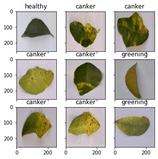
从加载图像到显示的完整代码如下:
|
1 2 3 4 5 6 7 8 9 10 11 12 13 14 15 16 17 18 19 20 |
from tensorflow.keras.utils import image_dataset_from_directory import matplotlib.pyplot as plt # 使用 image_dataset_from_directory() 加载图像,并将图像尺寸缩放为 256x256 PATH='.../Citrus/Leaves' # 修改为您的路径 ds = image_dataset_from_directory(PATH, validation_split=0.2, subset="training", image_size=(256,256), interpolation="mitchellcubic", crop_to_aspect_ratio=True, seed=42, shuffle=True, batch_size=32) # 从数据集中获取一个批次并显示图像 fig, ax = plt.subplots(3, 3, sharex=True, sharey=True, figsize=(5,5)) for images, labels in ds.take(1): for i in range(3): for j in range(3): ax[i][j].imshow(images[i*3+j].numpy().astype("uint8")) ax[i][j].set_title(ds.class_names[labels[i*3+j]]) plt.show() |
请注意,如果您使用 tensorflow_datasets 获取图像,样本将以字典形式而不是 (image,label) 元组的形式呈现。您需要对代码进行一些修改,如下所示:
|
1 2 3 4 5 6 7 8 9 10 11 12 13 14 15 16 17 |
import tensorflow_datasets as tfds import matplotlib.pyplot as plt # 使用 tfds.load() 或 image_dataset_from_directory() 加载图像 ds, meta = tfds.load('citrus_leaves', with_info=True, split='train', shuffle_files=True) ds = ds.batch(32) # 从数据集中获取一个批次并显示图像 fig, ax = plt.subplots(3, 3, sharex=True, sharey=True, figsize=(5,5)) for sample in ds.take(1): images, labels = sample["image"], sample["label"] for i in range(3): for j in range(3): ax[i][j].imshow(images[i*3+j].numpy().astype("uint8")) ax[i][j].set_title(meta.features['label'].int2str(labels[i*3+j])) plt.show() |
在本文的其余部分,假设数据集是使用 image_dataset_from_directory() 创建的。如果您的数据集创建方式不同,您可能需要对代码进行少量调整。
Keras 预处理层
Keras 包含许多神经网络层,例如您需要训练的卷积层。还有一些不带参数的层,例如将图像等数组展平为向量的 flatten 层。
Keras 中的预处理层专门设计用于神经网络的早期阶段。您可以使用它们进行图像预处理,例如调整图像大小、旋转图像或调整亮度和对比度。虽然预处理层应作为大型神经网络的一部分,但您也可以将它们用作函数。下面是一个如何将 resize 层用作函数来转换一些图像并将它们与原始图像并排显示的示例:
|
1 2 3 4 5 6 7 8 9 10 11 12 13 14 15 16 17 |
... # 创建一个 resizing 层 out_height, out_width = 128,256 resize = tf.keras.layers.Resizing(out_height, out_width) # 显示原始图像与调整大小后的图像 fig, ax = plt.subplots(2, 3, figsize=(6,4)) for images, labels in ds.take(1): for i in range(3): ax[0][i].imshow(images[i].numpy().astype("uint8")) ax[0][i].set_title("original") # 调整大小 ax[1][i].imshow(resize(images[i]).numpy().astype("uint8")) ax[1][i].set_title("resize") plt.show() |
图像的尺寸是 256x256 像素,resize 层会将其变为 256x128 像素。上述代码的输出如下: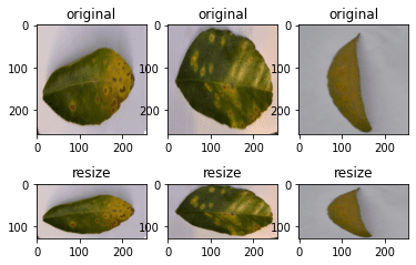
由于 resize 层是一个函数,您可以将其链式添加到数据集本身。例如:
|
1 2 3 4 5 6 7 8 |
... def augment(image, label): return resize(image), label resized_ds = ds.map(augment) for image, label in resized_ds: ... |
数据集 ds 的样本形式为 (image, label)。因此,您创建了一个接受这种元组并使用 resize 层进行图像预处理的函数。然后,您将此函数作为数据集的 map() 函数的参数。当您从使用 map() 函数创建的新数据集中抽取样本时,图像将是经过转换的。
还有更多的预处理层可用。其中一些演示如下。
如上所述,您可以调整图像大小。您还可以随机放大或缩小图像的高度或宽度。同样,您可以放大或缩小图像。下面是一个以最多增加或减少 30% 的方式操纵图像大小的示例:
|
1 2 3 4 5 6 7 8 9 10 11 12 13 14 15 16 17 18 19 20 21 22 23 24 25 26 27 28 29 |
... # 创建预处理层 out_height, out_width = 128,256 resize = tf.keras.layers.Resizing(out_height, out_width) height = tf.keras.layers.RandomHeight(0.3) width = tf.keras.layers.RandomWidth(0.3) zoom = tf.keras.layers.RandomZoom(0.3) # 可视化图像和增强效果 fig, ax = plt.subplots(5, 3, figsize=(6,14)) for images, labels in ds.take(1): for i in range(3): ax[0][i].imshow(images[i].numpy().astype("uint8")) ax[0][i].set_title("original") # 调整大小 ax[1][i].imshow(resize(images[i]).numpy().astype("uint8")) ax[1][i].set_title("resize") # 高度 ax[2][i].imshow(height(images[i]).numpy().astype("uint8")) ax[2][i].set_title("height") # 宽度 ax[3][i].imshow(width(images[i]).numpy().astype("uint8")) ax[3][i].set_title("width") # 缩放 ax[4][i].imshow(zoom(images[i]).numpy().astype("uint8")) ax[4][i].set_title("zoom") plt.show() |
这段代码显示图像如下: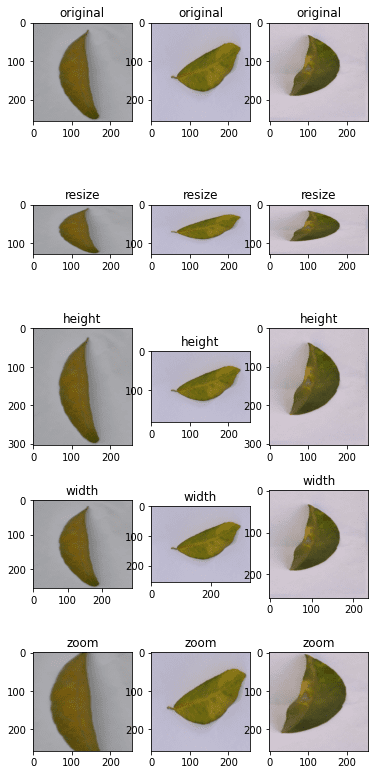
虽然您在 resize 中指定了固定的尺寸,但在其他增强操作中则具有随机的操纵量。
您还可以使用预处理层进行翻转、旋转、裁剪和几何平移。
|
1 2 3 4 5 6 7 8 9 10 11 12 13 14 15 16 17 18 19 20 21 22 23 24 25 26 27 |
... # 创建预处理层 flip = tf.keras.layers.RandomFlip("horizontal_and_vertical") # 或 "horizontal", "vertical" rotate = tf.keras.layers.RandomRotation(0.2) crop = tf.keras.layers.RandomCrop(out_height, out_width) translation = tf.keras.layers.RandomTranslation(height_factor=0.2, width_factor=0.2) # 可视化增强效果 fig, ax = plt.subplots(5, 3, figsize=(6,14)) for images, labels in ds.take(1): for i in range(3): ax[0][i].imshow(images[i].numpy().astype("uint8")) ax[0][i].set_title("original") # 翻转 ax[1][i].imshow(flip(images[i]).numpy().astype("uint8")) ax[1][i].set_title("flip") # 裁剪 ax[2][i].imshow(crop(images[i]).numpy().astype("uint8")) ax[2][i].set_title("crop") # 翻译 ax[3][i].imshow(translation(images[i]).numpy().astype("uint8")) ax[3][i].set_title("translation") # 旋转 ax[4][i].imshow(rotate(images[i]).numpy().astype("uint8")) ax[4][i].set_title("rotate") plt.show() |
此代码显示了以下图像: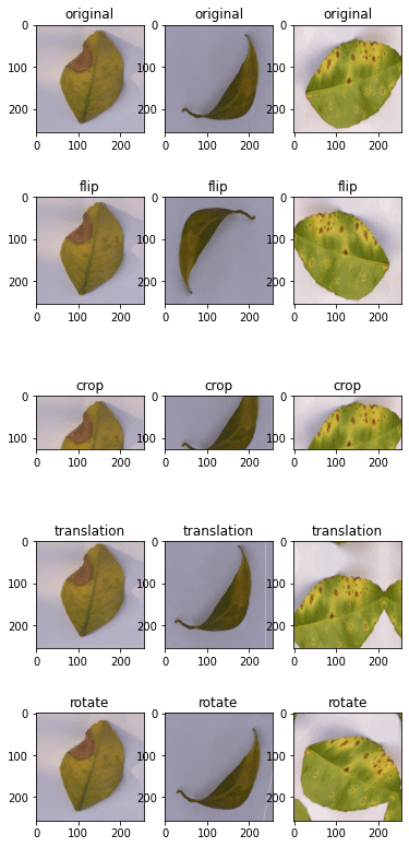
最后,您还可以对颜色调整进行增强
|
1 2 3 4 5 6 7 8 9 10 11 12 13 14 15 16 17 18 |
... brightness = tf.keras.layers.RandomBrightness([-0.8,0.8]) contrast = tf.keras.layers.RandomContrast(0.2) # 可视化增强 fig, ax = plt.subplots(3, 3, figsize=(6,7)) for images, labels in ds.take(1): for i in range(3): ax[0][i].imshow(images[i].numpy().astype("uint8")) ax[0][i].set_title("original") # 亮度 ax[1][i].imshow(brightness(images[i]).numpy().astype("uint8")) ax[1][i].set_title("brightness") # 对比度 ax[2][i].imshow(contrast(images[i]).numpy().astype("uint8")) ax[2][i].set_title("contrast") plt.show() |
这显示了如下图像: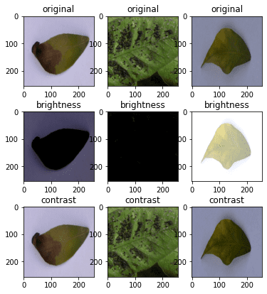
为了完整起见,以下是显示各种增强结果的代码
|
1 2 3 4 5 6 7 8 9 10 11 12 13 14 15 16 17 18 19 20 21 22 23 24 25 26 27 28 29 30 31 32 33 34 35 36 37 38 39 40 41 42 43 44 45 46 47 48 49 50 51 52 53 54 55 56 57 58 59 60 61 62 63 64 65 66 67 68 69 70 71 72 73 74 75 76 77 78 |
from tensorflow.keras.utils import image_dataset_from_directory import tensorflow as tf import matplotlib.pyplot as plt # 使用 image_dataset_from_directory() 加载图像,并将图像尺寸缩放为 256x256 PATH='.../Citrus/Leaves' # 修改为您的路径 ds = image_dataset_from_directory(PATH, validation_split=0.2, subset="training", image_size=(256,256), interpolation="mitchellcubic", crop_to_aspect_ratio=True, seed=42, shuffle=True, batch_size=32) # 创建预处理层 out_height, out_width = 128,256 resize = tf.keras.layers.Resizing(out_height, out_width) height = tf.keras.layers.RandomHeight(0.3) width = tf.keras.layers.RandomWidth(0.3) zoom = tf.keras.layers.RandomZoom(0.3) flip = tf.keras.layers.RandomFlip("horizontal_and_vertical") rotate = tf.keras.layers.RandomRotation(0.2) crop = tf.keras.layers.RandomCrop(out_height, out_width) translation = tf.keras.layers.RandomTranslation(height_factor=0.2, width_factor=0.2) brightness = tf.keras.layers.RandomBrightness([-0.8,0.8]) contrast = tf.keras.layers.RandomContrast(0.2) # 可视化图像和增强效果 fig, ax = plt.subplots(5, 3, figsize=(6,14)) for images, labels in ds.take(1): for i in range(3): ax[0][i].imshow(images[i].numpy().astype("uint8")) ax[0][i].set_title("original") # 调整大小 ax[1][i].imshow(resize(images[i]).numpy().astype("uint8")) ax[1][i].set_title("resize") # 高度 ax[2][i].imshow(height(images[i]).numpy().astype("uint8")) ax[2][i].set_title("height") # 宽度 ax[3][i].imshow(width(images[i]).numpy().astype("uint8")) ax[3][i].set_title("width") # 缩放 ax[4][i].imshow(zoom(images[i]).numpy().astype("uint8")) ax[4][i].set_title("zoom") plt.show() fig, ax = plt.subplots(5, 3, figsize=(6,14)) for images, labels in ds.take(1): for i in range(3): ax[0][i].imshow(images[i].numpy().astype("uint8")) ax[0][i].set_title("original") # 翻转 ax[1][i].imshow(flip(images[i]).numpy().astype("uint8")) ax[1][i].set_title("flip") # 裁剪 ax[2][i].imshow(crop(images[i]).numpy().astype("uint8")) ax[2][i].set_title("crop") # 翻译 ax[3][i].imshow(translation(images[i]).numpy().astype("uint8")) ax[3][i].set_title("translation") # 旋转 ax[4][i].imshow(rotate(images[i]).numpy().astype("uint8")) ax[4][i].set_title("rotate") plt.show() fig, ax = plt.subplots(3, 3, figsize=(6,7)) for images, labels in ds.take(1): for i in range(3): ax[0][i].imshow(images[i].numpy().astype("uint8")) ax[0][i].set_title("original") # 亮度 ax[1][i].imshow(brightness(images[i]).numpy().astype("uint8")) ax[1][i].set_title("brightness") # 对比度 ax[2][i].imshow(contrast(images[i]).numpy().astype("uint8")) ax[2][i].set_title("contrast") plt.show() |
最后,需要指出的是,大多数神经网络模型通过缩放输入图像可以获得更好的效果。虽然我们通常使用 8 位无符号整数作为图像中的像素值(例如,如上所示使用 imshow() 显示),但神经网络更倾向于将像素值保持在 0 到 1 或 -1 到 +1 之间。这也可以通过预处理层来实现。下面展示了如何更新上面的一些示例以将缩放层添加到增强中
|
1 2 3 4 5 6 7 8 9 10 11 12 |
... out_height, out_width = 128,256 resize = tf.keras.layers.Resizing(out_height, out_width) rescale = tf.keras.layers.Rescaling(1/127.5, offset=-1) # 将像素值重新缩放到 [-1,1] def augment(image, label): return rescale(resize(image)), label rescaled_resized_ds = ds.map(augment) for image, label in rescaled_resized_ds: ... |
使用 tf.image API 进行增强
除了预处理层之外,tf.image 模块还提供了一些用于增强的函数。与预处理层不同,这些函数旨在在用户定义的函数中使用,并通过 map() 分配给数据集,正如我们上面看到的。
tf.image 提供的函数不是预处理层的重复,尽管存在一些重叠。下面是一个使用 tf.image 函数来调整和裁剪图像的示例
|
1 2 3 4 5 6 7 8 9 10 11 12 13 14 15 16 17 18 19 20 21 22 23 24 25 26 27 28 |
... fig, ax = plt.subplots(5, 3, figsize=(6,14)) for images, labels in ds.take(1): for i in range(3): # 原始 ax[0][i].imshow(images[i].numpy().astype("uint8")) ax[0][i].set_title("original") # 调整大小 h = int(256 * tf.random.uniform([], minval=0.8, maxval=1.2)) w = int(256 * tf.random.uniform([], minval=0.8, maxval=1.2)) ax[1][i].imshow(tf.image.resize(images[i], [h,w]).numpy().astype("uint8")) ax[1][i].set_title("resize") # 裁剪 y, x, h, w = (128 * tf.random.uniform((4,))).numpy().astype("uint8") ax[2][i].imshow(tf.image.crop_to_bounding_box(images[i], y, x, h, w).numpy().astype("uint8")) ax[2][i].set_title("crop") # 中心裁剪 x = tf.random.uniform([], minval=0.4, maxval=1.0) ax[3][i].imshow(tf.image.central_crop(images[i], x).numpy().astype("uint8")) ax[3][i].set_title("central crop") # 随机裁剪到 (h,w) h, w = (256 * tf.random.uniform((2,))).numpy().astype("uint8") seed = tf.random.uniform((2,), minval=0, maxval=65536).numpy().astype("int32") ax[4][i].imshow(tf.image.stateless_random_crop(images[i], [h,w,3], seed).numpy().astype("uint8")) ax[4][i].set_title("random crop") plt.show() |
以下是上述代码的输出: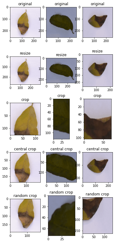
虽然图像显示与您对代码的预期相符,但 tf.image 函数的使用方式与预处理层截然不同。每个 tf.image 函数都是不同的。因此,您可以看到 crop_to_bounding_box() 函数接受像素坐标,而 central_crop() 函数则假设一个分数比例作为参数。
这些函数在处理随机性方面也不同。其中一些函数不假定随机行为。因此,随机调整大小应在调用 resize 函数之前使用随机数生成器单独生成确切的输出大小。其他一些函数,例如 stateless_random_crop(),可以随机进行增强,但需要显式指定一对 int32 类型的随机种子。
继续举例,这里有用于翻转图像和提取 Sobel 边缘的函数
|
1 2 3 4 5 6 7 8 9 10 11 12 13 14 15 16 17 18 19 20 21 22 23 |
... fig, ax = plt.subplots(5, 3, figsize=(6,14)) for images, labels in ds.take(1): for i in range(3): ax[0][i].imshow(images[i].numpy().astype("uint8")) ax[0][i].set_title("original") # 翻转 seed = tf.random.uniform((2,), minval=0, maxval=65536).numpy().astype("int32") ax[1][i].imshow(tf.image.stateless_random_flip_left_right(images[i], seed).numpy().astype("uint8")) ax[1][i].set_title("flip left-right") # 翻转 seed = tf.random.uniform((2,), minval=0, maxval=65536).numpy().astype("int32") ax[2][i].imshow(tf.image.stateless_random_flip_up_down(images[i], seed).numpy().astype("uint8")) ax[2][i].set_title("flip up-down") # sobel 边缘 sobel = tf.image.sobel_edges(images[i:i+1]) ax[3][i].imshow(sobel[0, ..., 0].numpy().astype("uint8")) ax[3][i].set_title("sobel y") # sobel 边缘 ax[4][i].imshow(sobel[0, ..., 1].numpy().astype("uint8")) ax[4][i].set_title("sobel x") plt.show() |
这显示了以下内容: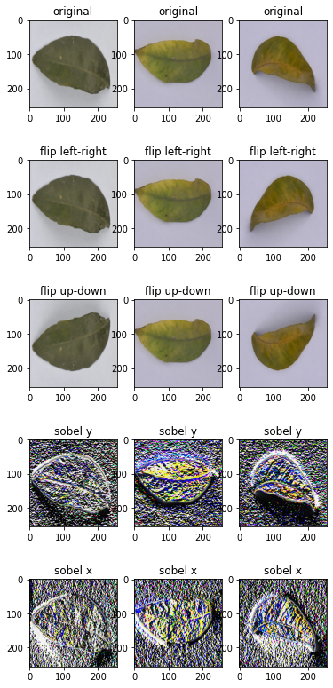
以下是用于处理亮度、对比度和颜色的函数
|
1 2 3 4 5 6 7 8 9 10 11 12 13 14 15 16 17 18 19 20 21 |
... fig, ax = plt.subplots(5, 3, figsize=(6,14)) for images, labels in ds.take(1): for i in range(3): ax[0][i].imshow(images[i].numpy().astype("uint8")) ax[0][i].set_title("original") # 亮度 seed = tf.random.uniform((2,), minval=0, maxval=65536).numpy().astype("int32") ax[1][i].imshow(tf.image.stateless_random_brightness(images[i], 0.3, seed).numpy().astype("uint8")) ax[1][i].set_title("brightness") # 对比度 ax[2][i].imshow(tf.image.stateless_random_contrast(images[i], 0.7, 1.3, seed).numpy().astype("uint8")) ax[2][i].set_title("contrast") # 饱和度 ax[3][i].imshow(tf.image.stateless_random_saturation(images[i], 0.7, 1.3, seed).numpy().astype("uint8")) ax[3][i].set_title("saturation") # 色调 ax[4][i].imshow(tf.image.stateless_random_hue(images[i], 0.3, seed).numpy().astype("uint8")) ax[4][i].set_title("hue") plt.show() |
此代码显示了以下内容: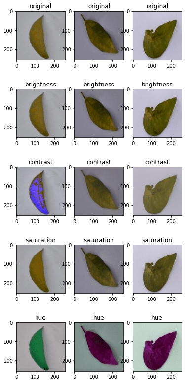
下面是显示以上所有内容的完整代码
|
1 2 3 4 5 6 7 8 9 10 11 12 13 14 15 16 17 18 19 20 21 22 23 24 25 26 27 28 29 30 31 32 33 34 35 36 37 38 39 40 41 42 43 44 45 46 47 48 49 50 51 52 53 54 55 56 57 58 59 60 61 62 63 64 65 66 67 68 69 70 71 72 73 74 75 76 77 78 79 80 81 |
from tensorflow.keras.utils import image_dataset_from_directory import tensorflow as tf import matplotlib.pyplot as plt # 使用 image_dataset_from_directory() 加载图像,并将图像尺寸缩放为 256x256 PATH='.../Citrus/Leaves' # 修改为您的路径 ds = image_dataset_from_directory(PATH, validation_split=0.2, subset="training", image_size=(256,256), interpolation="mitchellcubic", crop_to_aspect_ratio=True, seed=42, shuffle=True, batch_size=32) # 可视化 tf.image 增强 fig, ax = plt.subplots(5, 3, figsize=(6,14)) for images, labels in ds.take(1): for i in range(3): # 原始 ax[0][i].imshow(images[i].numpy().astype("uint8")) ax[0][i].set_title("original") # 调整大小 h = int(256 * tf.random.uniform([], minval=0.8, maxval=1.2)) w = int(256 * tf.random.uniform([], minval=0.8, maxval=1.2)) ax[1][i].imshow(tf.image.resize(images[i], [h,w]).numpy().astype("uint8")) ax[1][i].set_title("resize") # 裁剪 y, x, h, w = (128 * tf.random.uniform((4,))).numpy().astype("uint8") ax[2][i].imshow(tf.image.crop_to_bounding_box(images[i], y, x, h, w).numpy().astype("uint8")) ax[2][i].set_title("crop") # 中心裁剪 x = tf.random.uniform([], minval=0.4, maxval=1.0) ax[3][i].imshow(tf.image.central_crop(images[i], x).numpy().astype("uint8")) ax[3][i].set_title("central crop") # 随机裁剪到 (h,w) h, w = (256 * tf.random.uniform((2,))).numpy().astype("uint8") seed = tf.random.uniform((2,), minval=0, maxval=65536).numpy().astype("int32") ax[4][i].imshow(tf.image.stateless_random_crop(images[i], [h,w,3], seed).numpy().astype("uint8")) ax[4][i].set_title("random crop") plt.show() fig, ax = plt.subplots(5, 3, figsize=(6,14)) for images, labels in ds.take(1): for i in range(3): ax[0][i].imshow(images[i].numpy().astype("uint8")) ax[0][i].set_title("original") # 翻转 seed = tf.random.uniform((2,), minval=0, maxval=65536).numpy().astype("int32") ax[1][i].imshow(tf.image.stateless_random_flip_left_right(images[i], seed).numpy().astype("uint8")) ax[1][i].set_title("flip left-right") # 翻转 seed = tf.random.uniform((2,), minval=0, maxval=65536).numpy().astype("int32") ax[2][i].imshow(tf.image.stateless_random_flip_up_down(images[i], seed).numpy().astype("uint8")) ax[2][i].set_title("flip up-down") # sobel 边缘 sobel = tf.image.sobel_edges(images[i:i+1]) ax[3][i].imshow(sobel[0, ..., 0].numpy().astype("uint8")) ax[3][i].set_title("sobel y") # sobel 边缘 ax[4][i].imshow(sobel[0, ..., 1].numpy().astype("uint8")) ax[4][i].set_title("sobel x") plt.show() fig, ax = plt.subplots(5, 3, figsize=(6,14)) for images, labels in ds.take(1): for i in range(3): ax[0][i].imshow(images[i].numpy().astype("uint8")) ax[0][i].set_title("original") # 亮度 seed = tf.random.uniform((2,), minval=0, maxval=65536).numpy().astype("int32") ax[1][i].imshow(tf.image.stateless_random_brightness(images[i], 0.3, seed).numpy().astype("uint8")) ax[1][i].set_title("brightness") # 对比度 ax[2][i].imshow(tf.image.stateless_random_contrast(images[i], 0.7, 1.3, seed).numpy().astype("uint8")) ax[2][i].set_title("contrast") # 饱和度 ax[3][i].imshow(tf.image.stateless_random_saturation(images[i], 0.7, 1.3, seed).numpy().astype("uint8")) ax[3][i].set_title("saturation") # 色调 ax[4][i].imshow(tf.image.stateless_random_hue(images[i], 0.3, seed).numpy().astype("uint8")) ax[4][i].set_title("hue") plt.show() |
这些增强函数对于大多数用途来说已经足够了。但如果您对图像增强有具体的想法,可能需要一个更好的图像处理库。 OpenCV 和 Pillow 是常用的但功能强大的库,可以更好地转换图像。
在神经网络中使用预处理层
在上面的示例中,您将 Keras 预处理层用作函数。但它们也可以用作神经网络中的层。这非常简单。下面是如何将预处理层合并到分类网络中并使用数据集对其进行训练的示例
|
1 2 3 4 5 6 7 8 9 10 11 12 13 14 15 16 17 18 19 20 21 22 23 24 25 26 27 28 29 30 31 32 33 34 35 36 |
from tensorflow.keras.utils import image_dataset_from_directory import tensorflow as tf import matplotlib.pyplot as plt # 使用 image_dataset_from_directory() 加载图像,并将图像尺寸缩放为 256x256 PATH='.../Citrus/Leaves' # 修改为您的路径 ds = image_dataset_from_directory(PATH, validation_split=0.2, subset="training", image_size=(256,256), interpolation="mitchellcubic", crop_to_aspect_ratio=True, seed=42, shuffle=True, batch_size=32) AUTOTUNE = tf.data.AUTOTUNE ds = ds.cache().prefetch(buffer_size=AUTOTUNE) num_classes = 5 model = tf.keras.Sequential([ tf.keras.layers.RandomFlip("horizontal_and_vertical"), tf.keras.layers.RandomRotation(0.2), tf.keras.layers.Rescaling(1/127.0, offset=-1), tf.keras.layers.Conv2D(32, 3, activation='relu'), tf.keras.layers.MaxPooling2D(), tf.keras.layers.Conv2D(32, 3, activation='relu'), tf.keras.layers.MaxPooling2D(), tf.keras.layers.Conv2D(32, 3, activation='relu'), tf.keras.layers.MaxPooling2D(), tf.keras.layers.Flatten(), tf.keras.layers.Dense(128, activation='relu'), tf.keras.layers.Dense(num_classes) ]) model.compile(optimizer='adam', loss=tf.keras.losses.SparseCategoricalCrossentropy(from_logits=True), metrics=['accuracy']) model.fit(ds, epochs=3) |
运行上面的代码将产生以下输出
|
1 2 3 4 5 6 7 8 |
发现609个文件,属于5个类别。 使用488个文件进行训练。 Epoch 1/3 16/16 [==============================] - 5s 253ms/step - loss: 1.4114 - accuracy: 0.4283 Epoch 2/3 16/16 [==============================] - 4s 259ms/step - loss: 0.8101 - accuracy: 0.6475 Epoch 3/3 16/16 [==============================] - 4s 267ms/step - loss: 0.7015 - accuracy: 0.7111 |
在上面的代码中,您使用cache()和prefetch()创建了数据集。这是一种性能技术,允许数据集在神经网络训练时异步准备数据。如果数据集使用map()函数分配了其他增强功能,这将非常重要。
如果您移除RandomFlip和RandomRotation层,您会看到准确率有所提高,因为这会使问题更容易。但是,当您希望网络在各种图像质量和属性上都能很好地预测时,使用数据增强可以帮助您生成的网络更强大。
进一步阅读
以下是一些与上述示例相关的 TensorFlow 文档
总结
在这篇文章中,您已经看到了如何使用 tf.data 数据集与 Keras 和 TensorFlow 中的图像增强函数。
具体来说,你学到了:
- 如何使用 Keras 的预处理层,既作为函数又作为神经网络的一部分
- 如何创建自己的图像增强函数并使用
map()函数将其应用于数据集 - 如何使用
tf.image模块提供的函数进行图像增强


一篇非常有帮助的博文,但我对代码有 3 个问题。
问题 1:我必须将 TensorFlow 升级到 2.9.0 才能使 RandomBrightness 函数正常工作。
问题 2:当我运行您为最后一个示例创建的 Sequential 模型时,它抱怨模型的数据输入没有定义“shape”。查看模型时,我看不到您定义输入形状或输入数据的位置。这是在哪里完成的?
错误提示:“您必须提供
input_shape参数。”问题 3:我无法让以下代码工作
# 使用 image_dataset_from_directory() 加载图像,并将图像大小缩放到 256×256
PATH=’…/Citrus/Leaves’ # 修改为您的路径
ds = image_dataset_from_directory(PATH,
validation_split=0.2, subset=”training”,
image_size=(256,256), interpolation=”mitchellcubic”,
crop_to_aspect_ratio=True,
seed=42, shuffle=True, batch_size=32)
正如您所建议的,我必须用以下代码替换之前的代码才能使其他程序工作。
ds, meta = tfds.load(‘citrus_leaves’, with_info=True, split=’train’, shuffle_files=True)
ds = ds.batch(3*3)
for sample in ds.take(1)
images, labels = sample[“image”], sample[“label”]…
你好 Terry… 感谢您的反馈!您是手动输入代码示例还是复制粘贴的?另外,您是否尝试过在 Google Colab 中运行代码示例以排除本地 Python 环境可能存在的问题?
亲爱的 James,
在实现 “layers.experimental.preprocessing.RandomContrast(factor=0.8)” 时,我收到了以下错误
AdjustContrastv2 目前没有确定性的 GPU 实现。
[[{{node model/sequential_1/random_contrast/adjust_contrast}}]] [Op:__inference_train_function_3974]
有什么建议可以克服这个问题吗?由于这个错误,我无法运行
os.environ[‘TF_DETERMINISTIC_OPS’] = ‘1’
谢谢,顺祝商祺