在Keras中构建机器学习模型的三种方法

如果您在 GitHub 上查看过 Keras 模型，您可能已经注意到在 Keras 中创建模型有几种不同的方法。有一种是 Sequential 模型，它允许您在单行代码中定义整个模型，通常会添加一些换行以提高可读性。然后，还有函数式接口，它允许更复杂的模型架构，还有一个是 Model 子类，它有助于提高可重用性。本文将探讨在 Keras 中创建模型的不同方法，以及它们的优缺点。这将为您提供在 Keras 中构建自己的机器学习模型所需的知识。

完成本教程后，您将学到：

• Keras 提供的构建模型的不同方法
• 如何使用 Sequential 类、函数式接口以及继承 keras.Model 来构建 Keras 模型
• 何时使用不同的 Keras 模型创建方法

让我们开始吧！

在 Keras 中构建机器学习模型的三个方法
照片由 Mike Szczepanski 拍摄。保留部分权利。

概述

本教程分为三个部分，涵盖了在 Keras 中构建机器学习模型的不同方法

• 使用 Sequential 类
• 使用 Keras 的函数式接口
• 继承 keras.Model

使用 Sequential 类

Sequential 模型顾名思义。它由一系列层组成，一层接一层。根据 Keras 文档，

“Sequential 模型适用于简单的层堆叠，其中每层只有一个输入张量和一个输出张量。”

它是开始构建 Keras 模型的一种简单易用的方法。首先，导入 TensorFlow，然后导入 Sequential 模型

然后，您可以通过堆叠各种层来开始构建您的机器学习模型。在此示例中，让我们使用经典的 CIFAR-10 图像数据集作为输入来构建 LeNet5 模型

您会注意到，您只是将模型应包含的层数组传递给了 Sequential 模型构造函数。查看 model.summary()，您可以看到模型的架构。

为了测试模型，让我们加载 CIFAR-10 数据集并运行 model.compile 和 model.fit

这将产生如下输出：

对于初次尝试的模型来说，这已经相当不错了。将 LeNet5 使用 Sequential 模型的代码整合起来，您将得到：

现在，让我们看看构建 Keras 模型的其他方法可以做什么，首先是函数式接口！

使用 Keras 的函数式接口

您将探索的下一个构建 Keras 模型的方法是使用 Keras 的函数式接口。函数式接口将层用作函数，它们接收一个张量并输出一个张量。函数式接口是表示 Keras 模型的一种更灵活的方式，因为您不受限于只能创建堆叠在一起的层组成的顺序模型。相反，您可以构建分支成多个路径、具有多个输入的模型等。

考虑一个 Add 层，它接收来自两个或多个路径的输入并将张量相加。

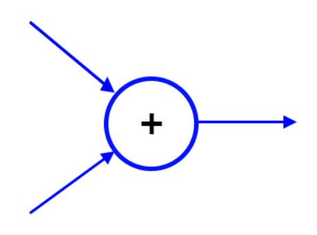
带有两个输入的 Add 层

由于无法通过顺序堆叠层来表示这种情况，因此您无法使用 Sequential 对象来定义它。这正是 Keras 函数式接口发挥作用的地方。您可以这样定义一个带有两个输入张量的 Add 层：

现在您已经看到了函数式接口的简短示例，让我们来看看使用函数式接口时，您通过实例化 Sequential 类定义的 LeNet5 模型会是什么样子。

查看模型摘要

正如你所见，你使用函数式接口或Sequential类实现的两种LeNet5模型的架构是相同的。

现在你已经了解了如何使用Keras的函数式接口，让我们来看一个可以使用函数式接口实现但不能用Sequential类实现的模型架构。本例中，我们将看残差块，它在ResNet中被提出。从视觉上看，残差块如下所示：

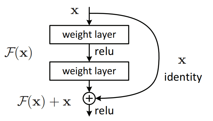
残差块，来源：https://arxiv.org/pdf/1512.03385.pdf

你可以看到，使用Sequential类定义的模型由于跳跃连接（skip connection）而无法构建这样的块，这使得该块无法表示为简单的层堆栈。使用函数式接口是定义ResNet块的一种方法。

然后，您可以使用函数式接口通过这些残差块构建一个简单的网络。

运行此代码并查看模型摘要和训练结果。

And combining the code for our simple network using residual blocks

继承 keras.Model

Keras also provides an object-oriented approach to creating models, which helps with reusability and allows you to represent the models you want to create as classes. This representation might be more intuitive since you can think about models as a set of layers strung together to form your network.

To begin subclassing keras.Model, you first need to import it

Then, you can start subclassing keras.Model. First, you need to build the layers that you want to use in your method calls since you only want to instantiate these layers once instead of each time you call your model. To keep in line with previous examples, let’s build a LeNet5 model here as well.

Then, override the call method to define what happens when the model is called. You override it with your model, which uses the layers you have built in the initializer.

It is important to have all the layers created at the class constructor, not inside the call() method. This is because the call() method will be invoked multiple times with different input tensors. But you want to use the same layer objects in each call to optimize their weight. You can then instantiate your new LeNet5 class and use it as part of a model

And you can see that the model has the same number of parameters as the previous two versions of LeNet5 that were built previously and has the same structure within it.

Combining all the code to create your LeNet5 subclass of keras.Model

进一步阅读

如果您想深入了解，本节提供了更多关于该主题的资源。

论文

• Deep Residual Learning for Image Recognition (the ResNet paper)

API

• Keras Sequential class
• Keras functional API
• Making new layers and models via subclassing

总结

In this post, you have seen three different ways to create models in Keras. In particular, this includes using the Sequential class, functional interface, and subclassing keras.Model. You have also seen examples of the same LeNet5 model being built using the different methods and a use case that can be done using the functional interface but not with the Sequential class.

具体来说，你学到了：

• Keras 提供的构建模型的不同方法
• 如何使用 Sequential 类、函数式接口以及继承 keras.Model 来构建 Keras 模型
• 何时使用不同的 Keras 模型创建方法